Introduction
GPU profiling is an exercise in narrowing uncertainty. Start with the outcome that matters, locate where its time goes, select the few kernels that can move that outcome, and only then collect expensive counters.
This book follows that order:
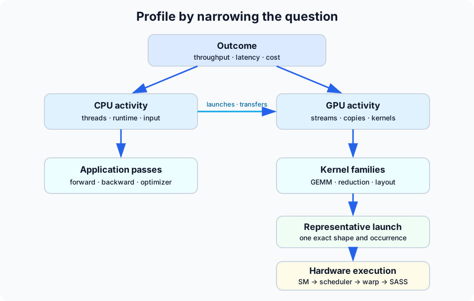
The most common profiling error is to begin at the bottom. A kernel can have poor occupancy (defined precisely in ch. 7), many stalls, or an ugly instruction mix and still be the wrong optimization target. Conversely, a kernel at 20% occupancy can be excellent if one deliberately large, warp-specialized block (ch. 10) saturates the relevant Tensor and memory pipelines (ch. 9–10). The vocabulary here is a preview; each term gets a full treatment once Part II reaches it.
What the tools answer
| Tool | Scope | Best question | Typical perturbation |
|---|---|---|---|
| Wall-clock benchmark | whole workload | Did the outcome improve? | very low |
| CUDA events | stream interval | How long did this GPU pass take? | low |
Nsight Systems (nsys) | CPU + GPU timeline | Is the GPU fed, and where are the gaps? | low to moderate |
Nsight Compute (ncu) | selected kernel launch | Why does this kernel take its time? | high; often multi-pass replay |
| Compiler reports / disassembly | one kernel image | What resources and instructions were emitted? | none at runtime |
A profiler's own overhead — injected instrumentation, replay passes, or sampling — can change the very timing it is trying to measure. "Perturbation" is how much a tool's presence distorts the number it reports, and it is why every measurement in this book is reported alongside the mechanism that produced it. The table above is also ordered cheap-to-expensive for a reason: a tool with high perturbation and long capture time, such as Nsight Compute replaying a kernel dozens of times to collect its counters, would be both too slow and too distorting to run across an entire application. That is exactly why the funnel in the next chapter starts with the cheapest, least-perturbing measurement and only escalates to a more invasive tool once a coarser one has narrowed the target.
A result is a claim plus evidence
A useful profile records:
- the workload and exact shapes;
- software, driver, and GPU versions;
- warm-up and synchronization boundaries;
- the measured distribution, not only its minimum;
- profiler settings and expected perturbation;
- a falsifiable next experiment.
Examples use standalone CUDA kernels and a representative mixed-precision transformer training workload. They are intended to teach reusable diagnoses, not a particular model architecture. Each diagnosis in Part II is also paired with the concrete technique that addresses it — coalescing and vectorized loads, software pipelining, warp specialization, register and precision trade-offs — so finishing a chapter means knowing not only what is slow, but what to change first.