13. Case studies
These case studies use a representative single-GPU, mixed-precision, approximately one-billion-parameter transformer training microstep. The batch contains 16 sequences of 1,024 predicted tokens. Activation checkpointing and CUDA Graph replay are enabled. The purpose is the diagnostic method; no knowledge of a particular model implementation is required.
Case A: thousands of launches, but not CPU-starved
A microstep launching several thousand kernels looks, on its face, like the textbook case for host-dispatch overhead — so that hypothesis is the one to rule in or out first, before trusting anything built on top of it. Ten graph replays contained 49,480 internal kernel nodes: 4,948 per microstep. The measured range was 12.810 s; the union was effectively serial and summed kernel time was 12.789 s. Device-idle time was therefore about 2.10 ms per microstep, or 0.164%.
| Observation | Superficial conclusion | Evidence-backed conclusion |
|---|---|---|
| 4,948 kernels/microstep | launch overhead must dominate | graph replay feeds them continuously |
long host cudaGraphLaunch calls | launch API is slow | calls block under queue backpressure while GPU runs |
| almost no device gap | — | CPU dispatch is not the current hot-path limit |
This does not prove the input pipeline will remain sufficient with real storage or distributed communication. It proves that kernel optimization, not further launch aggregation, controls this captured steady-state interval.
CUDA-event pass timing on the same shape makes the target more precise:
| Pass | Median stream time | Share | Median host enqueue time |
|---|---|---|---|
| backbone forward | 229.83 ms | 19.4% | 107.04 ms |
| fused vocabulary loss | 111.32 ms | 9.4% | 3.72 ms |
| backward + checkpoint recompute | 845.92 ms | 71.3% | 895.38 ms |
| total | 1,187.07 ms | 100% | — |
The host and stream columns are overlapping clocks, so they must not be added. Backward's long host enqueue interval says dispatch is close enough to monitor; the Systems trace's near-continuous GPU work says it is not presently opening meaningful device gaps. Backward and recompute own most of the optimization ceiling.
Whole-range GPU metric sampling supports the same conclusion:
| Sampled metric over three graph replays | Mean |
|---|---|
| graphics/compute engine active | 99.67% |
| at least one SM warp active | 93.29% |
| SM instruction issue | 19.02% |
| Tensor pipe active | 37.26% |
| compute warps in flight | 35.25% |
| DRAM read / write throughput | 33.89% / 21.84% |
| PCIe receive / transmit throughput | 0.22% / 1.01% |
The GPU is occupied, but the mixed workload does not continuously feed one execution pipe. Low PCIe activity also rules out host transfer bandwidth as the captured hot-path explanation. That low aggregate issue rate is a symptom, not a diagnosis — it describes no single kernel, and opening one of 4,948 launches at random would not explain it. It does not mean every kernel has 19% issue efficiency; it means the next step is to find where time actually concentrates before opening any one kernel.
Case B: identify the aggregate ceiling
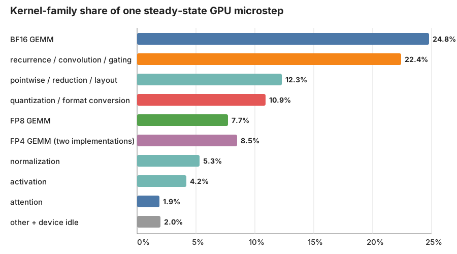
Attributing device time by kernel family, rather than by individual launch, answers that question directly: the workload is not dominated by one bad kernel. BF16 GEMMs are the largest family (24.8%), recurrent/convolution/gating kernels are close behind (22.4%), and format/layout work is distributed across pointwise and quantization families (23.2% combined).
Consequences from Amdahl's law:
- infinitely accelerating the recurrent family alone caps speedup at 1.289x;
- halving all quantization plus pointwise/layout work yields about 1.13x;
- reaching a 2.35x end-to-end target requires changing several large families or the hardware/parallelism, not polishing one kernel.
Format/layout and quantization work is one of those large families, and it is also the easiest to misjudge from a family label alone: on paper it looks like plain data movement, so the natural next question is whether it is actually copy traffic or compute wearing a copy's clothing.
Case C: “copy traffic” is mostly kernels
Quantization and pointwise/layout kernels made up nearly a quarter of the trace in Case B, so the question is what that share actually is. The trace showed only one small device copy per graph replay. By contrast, quantization kernels consumed 10.9%, and pointwise/reduction/layout kernels 12.3%. Two representative streaming kernels reached 88–89% DRAM throughput: a fused activation and a normalization kernel — each one is already efficient in isolation, so the excess time cannot be blamed on either kernel being slow.
The diagnosis is repeated read/transform/write passes, not a pathological
cudaMemcpyAsync. Useful experiments are fusion, reuse of quantized weights,
avoiding redundant layout materialization, or changing precision boundaries.
The activation arithmetic itself has little standalone ceiling when its kernel
already sits near the DRAM roof.
One FP4 packing kernel was different: 83% SM compute versus 35% DRAM, 100 registers/thread, and 33% theoretical occupancy. It is compute-heavy format conversion, so describing all quantization as “copying” would also be wrong.
That kernel's register count and occupancy are the first hint of a sharper, more specific problem than “too much traffic”: a kernel whose resource footprint limits how much work the SM can keep resident. The next case follows that thread to a single kernel where the full causal chain from registers to stalled scheduler cycles can be traced end to end.
Case D: maximum registers and spills are causal
A recurrent backward kernel represented 3.38% of the iteration by itself. It used 255 registers/thread with 128-thread blocks, achieved only eight warps/SM, generated 9.65 million local spill requests, and had no eligible warp on 91.6% of scheduler cycles. Long scoreboard accounted for 56% of its issue interval.
This is the clearest custom-kernel target because the causal chain is complete: register pressure reduces residency; spilling adds cache/memory dependencies; limited resident work cannot hide them; scheduler issue collapses. The first experiments should reduce live state or split a favorable phase—not impose a lower register cap.
A second backward kernel used 153 registers/thread, did not spill, achieved 25% occupancy, and reached 71% memory throughput. Its long-scoreboard latency is real, but it is a healthier, lower-priority memory-latency problem.
That contrast is worth generalizing before it is mistaken for a rule: low occupancy alone is not evidence of the first kernel's register/spill pathology. The next case checks that directly against two Tensor Core kernels that also run at moderate occupancy but are not register-limited at all.
Case E: low occupancy can be healthy
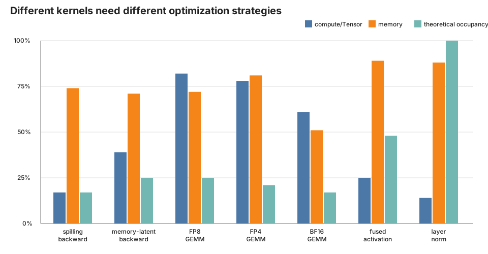
Neither depends on many resident warps to stay busy, so the question is whether their occupancy and stall numbers signal a problem to fix or a deliberate design already paying off. The FP8 GEMM reached about 82% Tensor-pipe utilization; the FP4 GEMM reached 78% Tensor and 81% memory/L2 throughput. Both deliberately ran one large, warp-specialized CTA per SM. Sleeping stalls represented producer/consumer waiting while the target pipelines remained busy.
The sampled grids also had efficient waves:
| Kernel | Grid CTAs | Assumed CTAs/SM | 84-SM wave efficiency |
|---|---|---|---|
| FP8 GEMM | 1,792 | 1 | 99.6% |
| FP4 GEMM | 4,736 | 1 | 98.9% |
| BF16 GEMM | 1,024 | 1 | 93.8% |
There is no evidence of a broad Tensor eligibility failure: the selected kernels execute Tensor instructions and saturate that pipe reasonably well. The BF16 sample is less efficient (61% Tensor, 51% DRAM, 16.7% occupancy) and shows math-pipe throttle without spills. Library tile selection and precision policy are more promising than rewriting the healthy FP8/FP4 kernels.
Cases A through E have now covered the aggregate picture and the specific kernel-level targets, both real (Case D) and illusory (Case E). One question remains that none of that kernel-level work answers: even capturing every identified gain, can this hardware reach the target at all?
Case F: feasibility before optimization
Answering that means comparing the measured rate against the actual target, not against intuition. The unprofiled steady-state baseline was approximately 14.08k tokens/s. A 20-tokens-per-parameter training budget for 1.0009B parameters is 20.018B tokens. Seven days therefore requires 33.10k tokens/s:
At the measured rate, the microstep-only lower bound is 16.45 days, before periodic optimizer, evaluation, checkpoint, or input costs. The gap is 2.35x. The profile shows no single-kernel route to that gain on this GPU. A realistic plan needs multiple GPUs or faster hardware, a smaller token/model budget, or a large algorithmic/precision redesign in addition to the identified kernel and fusion work.
None of that removes the value of the kernel and fusion targets identified in Cases B through E — it only bounds what they can accomplish alone. The final case runs those targets as an actual campaign and judges each one the way the rest of this book insists on: against whole-step time, not a counter in isolation.
Case G: a complete optimization campaign
The same representative workload was used for a controlled campaign. The important result is not that every plausible counter-driven edit won. It is that every edit was allowed to lose, and only whole-step improvements survived.
| Hypothesis | Experiment | Result | Decision |
|---|---|---|---|
| eliminate one residual-sized memory pass | fuse residual addition with the following prenorm | about +3.2% in isolation | retain after numerical gradient comparison |
| duplicate quantization is avoidable | share a common activation quantization across two projections while preserving separate GEMMs | about +1.6% in an adjacent pair | retain; the twice-wide single GEMM selected a slower shape |
| spare memory can buy compute | retain four tail layers instead of recomputing them | largest local gain, about +9% in the sweep | retain; eight layers exceeded memory |
| some precision-tail work is unnecessary | reduce a four-layer high-precision tail to two | about +2.6% versus four in the sweep | retain; deleting the tail entirely regressed |
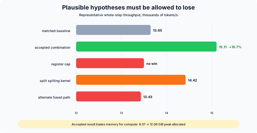
| occupancy is limited by 255 registers | cap registers at 128, 160, 192, and 224 | none beat uncapped | reject |
| spills justify splitting a backward kernel | materialize an intermediate between phases | numerically valid but slower | reject; added dot product and traffic outweighed spill savings |
The accepted changes interact, so their isolated percentages cannot be added. A matched 20-iteration comparison measured 13.65k versus 15.11k tokens/s:
Peak allocated memory rose from 9.07 to 12.06 GiB. That is not a regression in this experiment: memory below the device limit was intentionally exchanged for less recomputation. The decision would change if the production workload needed that headroom for optimizer state, communication buffers, or longer sequences.
The post-change graph made the traffic mechanism visible:
| Operation | Before / step | After / step | Change |
|---|---|---|---|
| common activation quantization | 120 | 84 | -30.0% |
| common transposed-activation quantization | 60 | 44 | -26.7% |
| all kernel nodes | 4,948 | 4,816 | -2.7% |
The small total launch-count change beside a large targeted count change is a useful reminder: the objective was not “fewer kernels.” It was fewer expensive full-tensor transformations while spending memory on avoided recomputation.
Finally, an instrumented post-change trace ran much slower than the unprofiled benchmark. Only bounded-range launch counts were compared across those reports; the end-to-end claim comes from matched unprofiled runs. This separation of evidence prevents profiler perturbation from becoming a false speedup or regression.
Read against the technique chapters, none of these six decisions is ad hoc.
Both accepted fusions — the residual/prenorm merge and the shared activation
quantization — are ch. 9's read-and-write elimination applied to concrete
GEMM neighbors once DRAM throughput was already high. The accepted
precision-tail reduction is ch. 8's Math Pipe Throttle lever of routing more
work onto a cheaper Tensor Core precision, bounded by ch. 10's dtype-eligibility
contract for whichever MMA path is actually available. Both rejections fail
for reasons the earlier chapters already flag: capping registers is the blind
-maxrregcount move ch. 7 warns against, and materializing an intermediate
between phases is exactly the kernel-split experiment ch. 7's spill diagnosis
suggests trying — it loses here because the added dot-product and traffic cost
is the accounting ch. 9 asks for before trusting a spill fix. The
warp-specialized FP8/FP4 GEMMs from Case E are what ch. 8's persistent-kernel
pattern and ch. 10's warp specialization look like once they are already
paying off, which is why this campaign's remaining slack was memory and
precision policy around them, not occupancy.