Introduction
GPU profiling is an exercise in narrowing uncertainty. Start with the outcome that matters, locate where its time goes, select the few kernels that can move that outcome, and only then collect expensive counters.
This book follows that order:
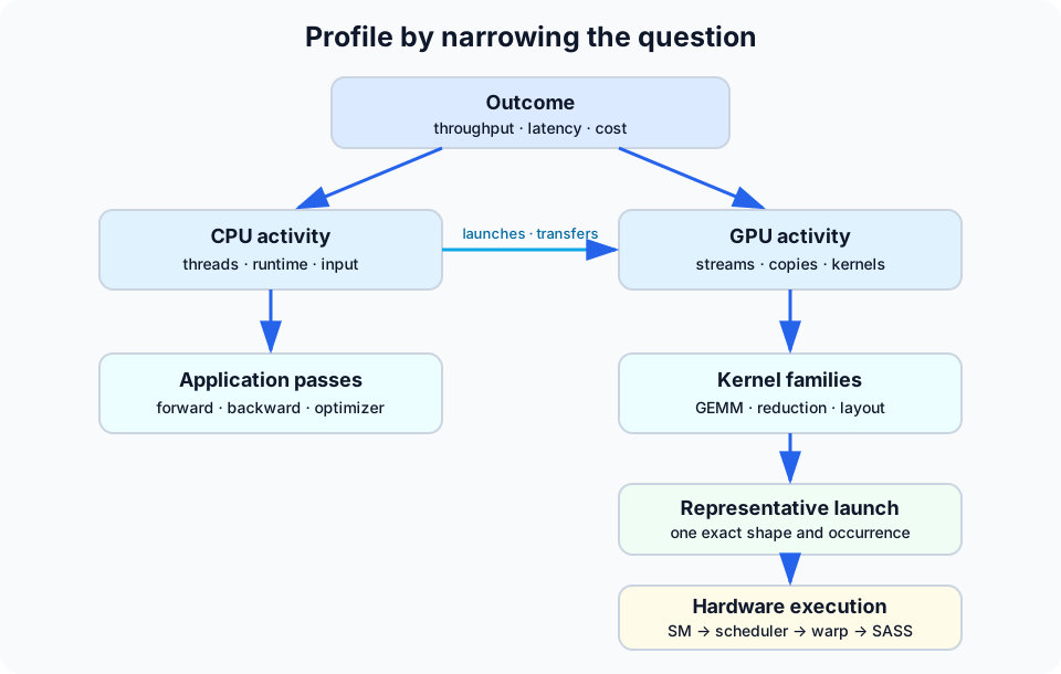
The most common profiling error is to begin at the bottom. A kernel can have poor occupancy (defined precisely in ch. 7), many stalls, or an ugly instruction mix and still be the wrong optimization target. Conversely, a kernel at 20% occupancy can be excellent if one deliberately large, warp-specialized block (ch. 10) saturates the relevant Tensor and memory pipelines (ch. 9–10). The vocabulary here is a preview; each term gets a full treatment once Part II reaches it.
What the tools answer
| Tool | Scope | Best question | Typical perturbation |
|---|---|---|---|
| Wall-clock benchmark | whole workload | Did the outcome improve? | very low |
| CUDA events | stream interval | How long did this GPU pass take? | low |
Nsight Systems (nsys) | CPU + GPU timeline | Is the GPU fed, and where are the gaps? | low to moderate |
Nsight Compute (ncu) | selected kernel launch | Why does this kernel take its time? | high; often multi-pass replay |
| Compiler reports / disassembly | one kernel image | What resources and instructions were emitted? | none at runtime |
A profiler's own overhead — injected instrumentation, replay passes, or sampling — can change the very timing it is trying to measure. "Perturbation" is how much a tool's presence distorts the number it reports, and it is why every measurement in this book is reported alongside the mechanism that produced it. The table above is also ordered cheap-to-expensive for a reason: a tool with high perturbation and long capture time, such as Nsight Compute replaying a kernel dozens of times to collect its counters, would be both too slow and too distorting to run across an entire application. That is exactly why the funnel in the next chapter starts with the cheapest, least-perturbing measurement and only escalates to a more invasive tool once a coarser one has narrowed the target.
A result is a claim plus evidence
A useful profile records:
- the workload and exact shapes;
- software, driver, and GPU versions;
- warm-up and synchronization boundaries;
- the measured distribution, not only its minimum;
- profiler settings and expected perturbation;
- a falsifiable next experiment.
Examples use standalone CUDA kernels and a representative mixed-precision transformer training workload. They are intended to teach reusable diagnoses, not a particular model architecture. Each diagnosis in Part II is also paired with the concrete technique that addresses it — coalescing and vectorized loads, software pipelining, warp specialization, register and precision trade-offs — so finishing a chapter means knowing not only what is slow, but what to change first.
1. The profiling funnel
Treat performance analysis as a sequence of gates. Do not move down a level until the current level identifies a question that the next tool can answer.
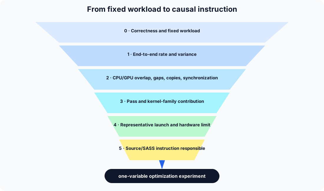
The optimization ceiling
Total runtime is the sum of every region's time, so no matter how much a chosen region is accelerated, everything outside it is an unmovable floor — this is why the chapter insists on estimating the ceiling before investing effort. If a region occupies fraction of runtime and is accelerated by , Amdahl's law gives the end-to-end speedup
Even deleting a 3% kernel completely yields only . Use this calculation before spending an afternoon on a visually dramatic counter. The ceiling is unforgiving at small shares and only becomes worth chasing once a region dominates the total:
| Share of time | 2x region speedup | Region removed entirely |
|---|---|---|
| 1% | 1.005x | 1.010x |
| 5% | 1.026x | 1.053x |
| 20% | 1.111x | 1.250x |
| 50% | 1.333x | 2.000x |
Decide which branch to follow
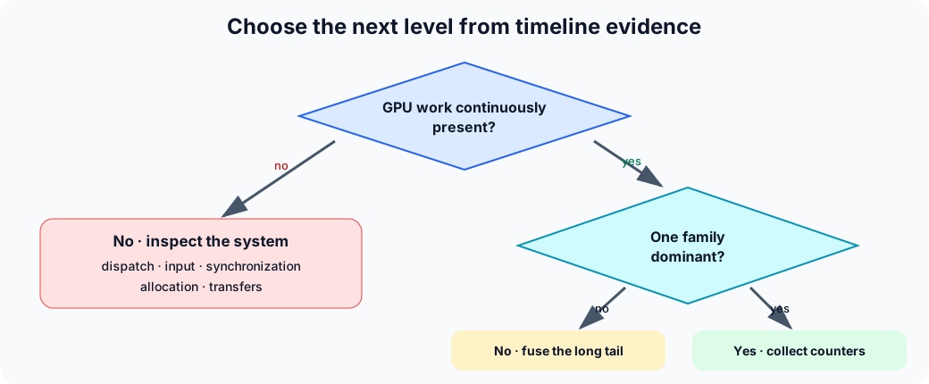
An iteration with thousands of kernels but less than 1% device idle time is not currently launch-starved. Graph capture (CUDA Graphs, covered in ch. 3) may have solved dispatch even though the graph still replays thousands of internal nodes. Keep host API duration and actual GPU idle gaps conceptually separate.
Evidence hierarchy
Prefer evidence in this order:
- repeatable end-to-end change;
- timeline change that accounts for it;
- counter change consistent with the timeline;
- compiler or SASS change that explains the counter;
- an intuition about what the hardware “should” do.
The last item is useful for forming hypotheses, not for declaring victory. Evidence closer to the top of this list is ranked higher because it is harder to fool yourself with: profiler overhead and measurement noise can produce an effect that looks real in a narrow, high-perturbation tool but disappears at the level that actually matters — unprofiled wall time.
2. Build a trustworthy baseline
Fix the experiment
Record the dimensions that change code generation or library selection. For a GEMM these are , layouts, dtype, epilogue (the post-accumulation step — bias, activation, scaling, store conversion), and alignment. For a model they include batch, sequence length, hidden sizes, precision policy, checkpointing, and graph/compile mode.
The primary rate is usually
where useful work may be tokens, images, requests, cells, or bytes. Define it so an optimization cannot “win” by silently doing less work.
Warm-up and timing
Warm-up must cover five effects, each of which makes the first iterations artificially slow for a distinct mechanical reason: lazy module loading (the CUDA driver does not load and link a kernel's binary until the first launch that needs it); JIT compilation (if the binary ships portable PTX instead of architecture-exact machine code, the driver compiles it to native instructions on first use, which is slow); autotuning (libraries like cuBLAS/cuDNN benchmark several internal kernel candidates on first call for a given shape and cache the winner); allocator growth (CUDA's caching memory allocator requests new device memory from the driver the first time a size is needed, which is far slower than reusing an already-grown pool); and cache creation (persistent kernels, workspaces, and lookup tables get built once and reused thereafter). Then synchronize around the measured region:
for (int i = 0; i < warmup; ++i) step();
cudaDeviceSynchronize();

auto t0 = std::chrono::steady_clock::now();
for (int i = 0; i < iterations; ++i) step();
cudaDeviceSynchronize();
auto t1 = std::chrono::steady_clock::now();
CUDA events measure elapsed device-stream time without turning every operation into a host synchronization:
cudaEventRecord(start, stream);
step(stream);
cudaEventRecord(stop, stream);
cudaEventSynchronize(stop);
cudaEventElapsedTime(&milliseconds, start, stop);
Use wall time for end-to-end truth and events to decompose GPU work. They answer different questions. CUDA calls are asynchronous — the host thread returns as soon as work is enqueued, not when it finishes — so host-side wall-clock timing around an individual call mostly measures dispatch latency. CUDA events are timestamps recorded directly on the GPU stream by the hardware and driver, so they measure real device execution time without forcing a host synchronization for every call.
Report a distribution
A single number hides variance from thermal state, OS scheduling, and contention. Report enough of the distribution that a reader can judge whether a change is real:
| Statistic | Why keep it |
|---|---|
| median | robust center for stable iterations |
| p20 / p80 or p10 / p90 | variance and thermal/OS effects |
| minimum | useful approximation to an interference-free lower bound |
| first iteration | exposes initialization; do not mix with steady state |
Locking clocks can reduce noise, but it changes the operating regime. If clocks
are not locked, record sampled clocks and compare utilization ratios more than
single-run nanoseconds in replayed ncu captures.
Baseline checklist
Capture the environment alongside the numbers, since driver, clock state, and topology all shift results without changing the code:
nvidia-smi --query-gpu=name,driver_version,pstate,clocks.sm,clocks.mem,\
temperature.gpu,power.draw,memory.total --format=csv
ncu --version
nsys --version
Also record CPU model, NUMA topology, memory capacity, framework/toolkit versions, and whether the environment is native Linux, Windows, a container, or WSL. Host scheduling and profiler permissions differ materially across them.
Capacity is part of performance
Track peak allocated and reserved device memory. Host or unified-memory spill can make a configuration appear to “run” while reducing throughput by orders of magnitude. A valid baseline states whether the complete steady-state workload, including optimizer state and periodic passes, fits.
3. Read the whole-system timeline
Nsight Systems answers when work occurs and what was waiting. It does not explain the instruction-level reason a kernel is slow.
Nsight Systems does not run your program instruction-by-instruction. It attaches to the CUDA driver and runtime through CUPTI (the CUDA Profiling Tools Interface) callbacks that fire whenever your program calls into CUDA — kernel launches, memory copies, stream and event operations — timestamping each one, while separately sampling OS-level thread and call-stack state (via OS scheduler and backtrace sampling) to see what the CPU is doing between those calls. It then merges both streams — the timestamped CUDA API/activity records and the sampled CPU state — into the single timeline you read in the viewer. This is why its overhead is comparatively low: it is mostly recording API calls that already happen and periodically sampling, not injecting deep instrumentation into every instruction. That low, roughly constant overhead is also why it is safe to run broadly and first, unlike Nsight Compute, whose kernel replay is invasive enough that it must be pointed at a small, already-identified target.
Instrument application semantics with NVTX
Ranges should describe coarse work: iteration, data load, forward, loss, backward, optimizer, communication, and checkpoint. Avoid marking every tiny operation.
#include <nvtx3/nvToolsExt.h>

nvtxRangePushA("iteration");
nvtxRangePushA("forward");
forward();
nvtxRangePop();
nvtxRangePushA("backward");
backward();
nvtxRangePop();
nvtxRangePop();
For Python frameworks, use their NVTX range context or direct NVTX bindings. Warm up outside the capture range.
An NVTX push/pop call just stamps a named, timestamped marker into the
CPU-side record for the profiler to display as a labeled row — it performs no
GPU work and adds negligible CPU cost, unlike the tracing and counter
collection nsys itself does on the CUDA API and kernel activity. That
asymmetry is why NVTX ranges are cheap enough to leave in near-production
code even when broader profiling is not running.
Start with a bounded trace
Open with a single, broad capture before narrowing to any specific concern:
nsys profile \
  --trace=cuda,nvtx,osrt \
  --sample=process-tree \
  --cpuctxsw=process-tree \
  --cuda-graph-trace=node \
  --output=timeline \
  ./application --profile-steps 5
A CUDA Graph captures a sequence of GPU operations and their dependencies once, then replays that whole sequence with a single launch call, amortizing host dispatch overhead across every node in the graph — this replay mechanism is the evidence behind Case A in the case studies (ch. 13). Node-level CUDA Graph tracing is useful when the graph's internal kernel mix is the subject of analysis, but it produces more data and overhead than graph-level tracing. Capture only enough steady-state iterations to see repetition.
Read the timeline top-down
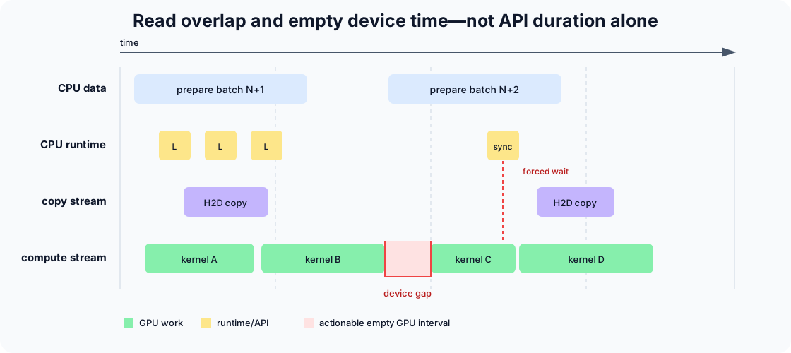
Ask these questions in order:
- Are there GPU-idle gaps inside the steady-state range?
- Is a CPU thread runnable, descheduled, blocked in a CUDA API, or doing data work during each gap?
- Are copies serialized with compute or placed on independent streams?
- Are allocations, page faults,
.item()-like scalar reads, or device-wide synchronizations present? - Is work balanced across streams/devices?
- Does the pattern repeat, or is it a one-time initialization event?
Interpret CUDA API time carefully
A long cudaGraphLaunch, cudaMemcpyAsync, or kernel-launch API call does not
automatically mean the API itself consumed that time as overhead. The call can
block under driver queue backpressure while previously submitted GPU work is
running. Confirm a host bottleneck with device-idle gaps and the corresponding
CPU state. Match the observed combination against a short set of recurring
patterns:
| Timeline pattern | Likely interpretation | Next check |
|---|---|---|
| GPU gaps; CPU executing framework code | dispatch/input bottleneck | CPU samples, Python backtraces, graphs/compile |
| GPU gaps; CPU blocked on sync API | accidental dependency | API backtrace, scalar reads, allocator |
| continuous kernels; CPU blocked in launch | queue backpressure, not starvation | device utilization and gaps |
| large H2D/D2H bands | explicit transfer or migration | bytes, direction, pinned memory, overlap |
| no copy bands but high DRAM traffic | kernels streaming data | Nsight Compute memory sections |
CLI summaries
Turn the same capture into ranked numbers instead of scrolling the timeline:
nsys stats --report cuda_gpu_kern_sum,cuda_gpu_mem_time_sum timeline.nsys-rep
nsys stats --report cuda_api_sum,nvtx_sum timeline.nsys-rep
Use summaries to rank kernel families, but return to the timeline for causality. Summed kernel durations can exceed wall time when streams overlap.
4. Attribute time to application passes
The system trace tells you whether the GPU is fed. Pass attribution tells you which semantic phase owns the work.
Use nested ranges and CUDA events
A training iteration might be segmented as:
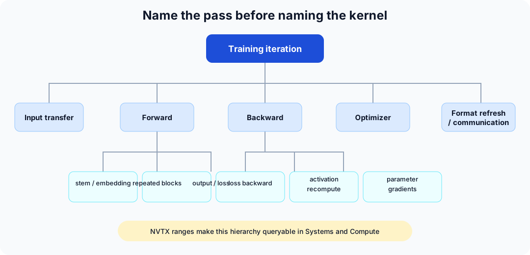
Put CUDA events at boundaries on the same stream for device elapsed time. Also measure host wall time around enqueueing. Never infer GPU pass time from Python function duration without an explicit synchronization or event. Operations enqueued on one stream execute in submission order, so an event timestamp reflects true completion order relative to the surrounding work on that stream, which is why same-stream events give trustworthy elapsed device time. Python-side wall time around a call is unreliable for the same reason it is unreliable elsewhere in this book: the call is asynchronous, so the host thread returns immediately after enqueueing, and unsynced wall time around it measures dispatch latency, not execution time.
Checkpointing changes the meaning of “backward”
With activation checkpointing, backward contains recomputed forward kernels. Categorizing only by kernel name can therefore overstate the original forward and hide recompute tax. NVTX ranges emitted by the autograd engine or explicitly timed pass boundaries preserve the causal phase.
For total forward time , backward work , and recomputed fraction , a rough iteration model is
Measure rather than assume ; custom recurrence, reductions, quantization, and fused loss kernels break simple FLOP models.
Kernel-family bucketing
Normalize long templated kernel names into meaningful families. Preserve enough metadata to distinguish materially different shapes.
| Raw launch property | Useful normalized field |
|---|---|
| demangled name | family: GEMM, norm, reduction, attention, quantize |
| grid/block | problem/tile class |
| registers and shared memory | resource signature |
| enclosing NVTX range | application pass |
| launch count and total time | optimization impact |
Report both total duration and launch count. A 10% family made of 2,000 tiny kernels suggests fusion or graph capture; a 10% family made of two long kernels suggests kernel-level work.
Quantify gaps
For a serial device interval,
This simple subtraction is invalid when streams overlap. In that case compute the union of occupied intervals, or use timeline recipes that account for concurrency.
The same accounting matters even when the launch count alone looks alarming. An observed graph-replayed training microstep in the case studies contained 4,948 internal kernel launches but only 0.16% device-idle time. The launch count looked alarming; the timeline showed that CPU dispatch was no longer the active limit.
5. Select kernels by impact
Nsight Compute can replay one launch dozens of times. Profile a small,
representative set rather than attaching --set full to an entire application.
Rank by contribution, then by distinct behavior
For each kernel family, compute
Select the largest contributors, then sample separate resource signatures or shapes within a family. A GEMM family with four shapes may need four samples; 800 identical elementwise launches usually need one.
| Selection criterion | Why it matters |
|---|---|
| high total time | end-to-end ceiling |
| long individual duration | stable counter sampling |
| high launch count | fusion/dispatch opportunity |
| unusual register/shared-memory signature | different occupancy regime (ch. 7) |
| different shape or tail wave (grid wave efficiency, ch. 10) | different tile efficiency |
| regression between revisions | direct causal target |
Preserve the production context
Ranking picks which kernel to profile; it says nothing about which invocation of that kernel is representative. The same symbol can behave differently with different shapes, alignment, cache state, concurrent streams, clocks, or data distributions. Prefer capturing a production launch with a kernel-name, NVTX, or launch-index filter. Use a standalone reproducer only after verifying its launch metadata and duration match the original.
Estimate the upper bound first
Before spending engineering time on a captured kernel, bound what fixing it can possibly buy. If family share is , a miraculous 2x kernel speedup produces only
That kernel may still be worth fixing if the same defect appears across related kernels, but the argument must be aggregate.
Avoid these selection traps
Even a disciplined ranking process fails in predictable ways:
- Profiling the first matching launch, which is often initialization or a small shape.
- Choosing the kernel with the lowest occupancy instead of the largest impact.
- Combining forward, backward, and recompute launches under one average.
- Comparing raw replay durations collected at substantially different clocks.
- Treating a library kernel's long C++ template name as a unique workload.
The nsys trace is the index into ncu: record the base symbol, occurrence,
grid, block, registers/thread, dynamic shared memory, stream, and enclosing
range before collecting counters.
6. A disciplined Nsight Compute workflow
Nsight Compute explains one selected kernel using launch metadata, static analysis, hardware counters, and PC sampling — periodically recording which instruction (program counter) each active warp was on and why it wasn't issuing that cycle, building a statistical map of where a kernel's time and stalls concentrate without recording every single cycle.
To build that picture, Nsight Compute pauses execution at one selected kernel
launch and reads hardware performance counters: physical counter circuits
built into each SM and into the memory subsystem that increment whenever a
specific hardware event occurs — an instruction issued on a given pipe, a
cache miss, a cycle a scheduler spent with no eligible warp of a particular
stall type. Each SM has only a limited number of these physical counters, and
many metrics either compete for the same counter hardware or are otherwise
mutually exclusive to collect in a single pass. Replay exists to work around
that limit; it is not just an implementation detail of "how ncu reruns a
kernel," it is the reason multiple passes exist at all. A --set full report
can be dozens of real kernel executions stitched together, each pass
collecting a different subset of counters, with device memory saved and
restored between passes so every pass sees the same input state and produces
counter values that are comparable with one another. This is also the root
cause of a fact the next section states directly: raw ncu duration does not
match the nsys timeline duration, because the kernel being timed in an ncu
report executed multiple times, in isolation, under replay control — not once,
in its original place alongside everything else on the timeline.
Capture in layers
Start cheap and escalate only as needed:
# Static launch data plus a small counter set
ncu --set basic \
    --kernel-name-base function \
    --kernel-name 'regex:my_kernel' \
    --launch-count 1 \
    -o my_kernel_basic \
    ./application

# Broader diagnosis
ncu --set detailed --kernel-name 'regex:my_kernel' --launch-count 1 \
    -o my_kernel_detailed ./application

# Expensive, multi-pass evidence after the launch is known to be stable
ncu --set full --kernel-name 'regex:my_kernel' --launch-count 1 \
    -o my_kernel_full ./application
Use --launch-skip N to reach a later matching occurrence. Filters count
matching launches, whereas --launch-skip-before-match counts all launches.
Inspect ncu --help for the exact NVTX range syntax supported by the installed
version.
Replay changes execution
Many metrics cannot be collected simultaneously. Kernel replay restores memory and runs the selected kernel in multiple passes. Consequences include:
- raw duration may not match the
nsystimeline; - cache and residency state may change;
- nondeterministic or stateful kernels may need application replay (reruns the whole program) or range replay (reruns only a marked range) instead, when kernel replay's memory restore is not safe;
- host memory backup can be expensive for kernels touching large allocations;
- uncontrolled clocks can differ between reports.
Use the Systems duration for contribution and the Compute report for the kernel's performance character. If raw timing is important, use a dedicated benchmark with stable clocks and minimal counter collection.
Read sections in a fixed order
Once a report is captured, the biggest risk is reading it out of order — jumping straight to the most dramatic number instead of building up resource and issue context first.
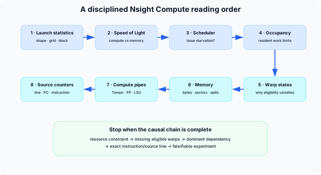
Do not begin with stall percentages. NVIDIA's own guidance is to focus on stalls when schedulers fail to issue; a busy scheduler can accumulate benign stall samples among warps it did not choose.
The four-way first classification
With reading order fixed, use memory and compute pressure together for a first-pass classification:
| Observation | Working classification | Confirm with |
|---|---|---|
| high DRAM/L2, low compute | bandwidth or memory-latency limited | bytes, hit rates, sectors, scoreboard |
| high Tensor/FP pipe | compute-pipe limited | math throttle, instruction mix |
| both high | well balanced near roof | roofline, end-to-end share |
| both low | latency, dependencies, insufficient parallelism, tails | eligible warps, waves, occupancy, stalls |
“High” is architectural and workload dependent. Use achieved percentage of the relevant peak, not a universal 80% rule.
Eligible warps and stalls (ch. 8), occupancy (ch. 7), and wave/tail efficiency (ch. 10) each get their own chapter. Treat this table as the dispatcher that tells you which of those chapters to open next, not as a definition of the terms themselves.
Export reports reproducibly
Once a report supports a working classification, preserve it rather than re-deriving it from a narrow export:
ncu --import my_kernel_full.ncu-rep --page details --csv
Keep the binary .ncu-rep; the UI includes rooflines, source correlation, and
occupancy what-if controls that a narrow CSV export cannot reproduce.
7. Occupancy, registers, and spills
Occupancy is resident active warps divided by the architectural maximum. It is a latency-hiding resource, not a performance score.
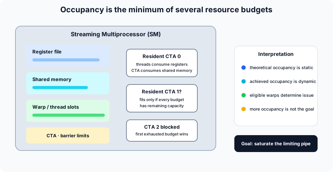
GPUs cannot make a DRAM read finish faster; a round trip to device memory still takes hundreds of cycles no matter how the kernel is written. Instead, an SM hides that latency by keeping many warps resident at once, so that when one warp's next instruction has an unmet dependency — an operand not yet computed, a value not yet returned from memory — the scheduler can switch to issuing an instruction from a different, already-ready warp on the very next cycle instead of leaving the pipeline idle. Occupancy measures how much of that switching inventory is present. This is why the book calls it "latency-hiding" rather than "more parallelism is always better": once enough resident warps exist to keep the scheduler supplied with an eligible one on every cycle, additional occupancy has nothing left to hide and stops helping, while forcing it higher can even cost performance if it comes at the expense of registers or shared memory a kernel needed for something else (the warp-specialized GEMM later in this chapter is a case where low occupancy is by design). Occupancy has a ceiling because only a finite number of thread slots, warp slots, registers, and shared-memory bytes exist per SM; whichever of those four resources is exhausted first caps how many warps can be simultaneously resident. The formula below computes exactly that bound, one term per resource.
Resource limits combine
For threads/block , warps/block , registers per thread , and shared memory per block , an approximate block limit is
Real register and shared-memory allocation is rounded in architecture-specific granularities, so use Nsight Compute's occupancy section/calculator for exact limits.
Read theoretical and achieved occupancy together
Theoretical occupancy is a ceiling computed from resources; it says nothing about whether that ceiling is reached or whether reaching it would even help. Compare theoretical against achieved before drawing a conclusion:
| Pattern | Interpretation |
|---|---|
| theoretical low, achieved near theoretical | launch resource limit is real |
| theoretical high, achieved much lower | tails, imbalance, short kernel, or sampling artifact |
| low occupancy, high target-pipe utilization | likely sufficient or deliberate |
| low occupancy, low issue rate, long dependency stalls | latency hiding is insufficient |
On a warp-specialized GEMM, one 384-thread CTA may intentionally consume about 80–90 KiB shared memory and 168 registers/thread. One CTA/SM can still keep the Tensor pipe near saturation. Reducing registers simply to raise occupancy can slow it down by breaking the software pipeline.
Registers versus local memory
“Local” memory is thread-private in the programming model but physically lives in device memory and is cached. Compiler-generated stack slots, arrays with dynamic indexing, and spilled live values use it.
Compile CUDA code with resource reporting and line information:
nvcc -O3 -lineinfo -Xptxas=-v kernel.cu -o kernel
Then inspect in Nsight Compute:
- Registers Per Thread;
- Local Memory Total;
- local load/store instructions and sectors;
- L1/L2 sectors attributable to local traffic;
- source lines with local-memory instructions.
A register-spill diagnosis
Put registers, local memory, and occupancy together on one concrete kernel. Consider a 128-thread backward kernel using 255 registers/thread. Its stall profile is dominated by long-scoreboard stalls (waiting on an L1TEX-tracked memory result; the full stall taxonomy follows in ch. 8):
| Metric | Observation |
|---|---|
| theoretical / achieved occupancy | 16.67% / 16.62% |
| active warps per SM | 7.98 |
| register block limit | 2 CTAs |
| local spill requests | 9.65 million |
| scheduler cycles with no eligible warp | 91.6% |
| long-scoreboard share | 56% of issue interval |
Registers limit residency and the kernel still spills. This is not an
argument to apply -maxrregcount blindly—that usually creates more spills. It
is evidence to reduce live ranges, recompute cheap intermediates, shrink
per-thread tiles, reorganize state, or split the kernel at a boundary with a
favorable intermediate size.
Safe experiments
Turn that evidence into experiments, one variable at a time:
- Inspect the exact SASS/source lines producing local traffic.
- Change one tile/live-state parameter.
- Verify numerical behavior.
- Re-check registers, spills, occupancy, and duration together.
- Measure the complete workload.
Step 2 covers more than shrinking a tile size. One concrete version of it is the kernel split already named above: splitting the kernel at a boundary with a favorable intermediate size trades one extra read/write pass — the intermediate now has to be written out and read back in — for lower live range per thread and, potentially, higher occupancy in each half. That tradeoff is not free, and it is not automatically favorable. Ch. 13's Case G tried exactly this hypothesis on this exact kernel: materializing an intermediate between phases of the backward pass was numerically valid and did lower register pressure, but it ran slower — the added memory traffic from writing and re-reading the intermediate outweighed the spill savings it was meant to buy. Treat a kernel split the same way as any other step-2 change: a hypothesis to run through the full ledger discipline from ch. 12, not a technique that pays off just because it addresses the diagnosis on paper.
__launch_bounds__ and maximum-register flags are experiments, not fixes. A
higher occupancy number is a win only if relevant elapsed time falls.
8. Schedulers, stalls, and execution pipes
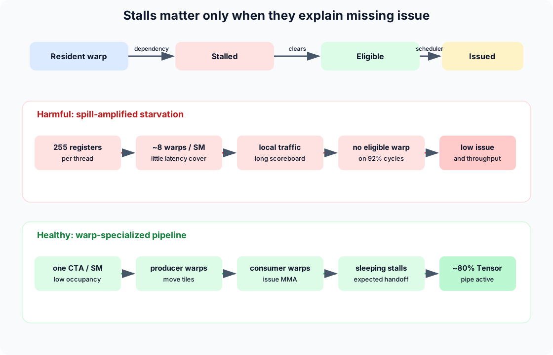
Each SM has warp schedulers. On a cycle, a scheduler chooses an eligible warp and issues its next instruction. A warp is 32 threads executing the same instruction together in lockstep (SIMT); "issuing an instruction" for a warp means all 32 lanes step forward together. A warp may be active but ineligible because an operand, pipeline, barrier, or memory dependency is not ready — it is "not eligible" precisely when the next instruction it needs to run still has an unmet dependency: an operand not yet computed, a memory value not yet returned, a barrier not yet reached.
Start with scheduler health
| Metric | Question |
|---|---|
| active warps/scheduler | how much latency-hiding inventory exists? |
| eligible warps/scheduler | how many can issue now? |
| issued warps/scheduler | how often does useful issue occur? |
| no eligible (%) | how often is the scheduler starved? |
| issue slots busy | is instruction issue itself well utilized? |
Only after establishing poor issue efficiency should stall reasons dominate the investigation.
Common stall reasons
Names vary slightly by architecture and tool release; use the installed Profiling Guide for exact definitions.
| Stall | Usually means | Productive experiments |
|---|---|---|
| Long Scoreboard | wait for L1TEX-tracked memory result, often global/local | coalescing, cache reuse, prefetch, more independent work/warps |
| Short Scoreboard | shorter MIO/shared-memory dependency | shared layout, bank conflicts, scheduling |
| Math Pipe Throttle | target arithmetic pipe is saturated | reduce operations, use faster precision/pipe, improve tiling |
| MIO Throttle | LSU/SFU/shared/branch issue pressure | simplify addressing, redistribute instruction mix |
| Barrier | CTA/warp synchronization imbalance | reduce barriers, balance producer/consumer work |
| Wait | fixed-latency dependency or explicit wait | add independent instructions, pipeline stages |
| Sleeping | nanosleep or deliberate producer/consumer backoff | often normal in persistent/warp-specialized kernels |
| Not Selected | another eligible warp issued | generally healthy if issue slots are busy |
| Branch Resolving / Divergence | control-flow dependency or lane disagreement | predication, regroup work, uniform branches |
Turning a stall diagnosis into a fix
The table above names a direction — "coalescing," "reduce operations," "predication" — but a direction is not yet a technique. This section fills in the concrete mechanism behind each stall category's productive experiments, so a diagnosis has somewhere specific to go.
Long Scoreboard and MIO Throttle (memory-bound stalls). If a warp is
repeatedly stalling because its next instruction needs a value that has not
come back from memory yet, the instruction stream is asking for data too
late relative to when it is used. Software pipelining, also called
double buffering, restructures the loop so the load for tile is
issued before the compute on tile finishes, using a second buffer (a
second shared-memory tile or register set) so the two tiles do not collide.
The warp then has independent work — compute on the already-resident tile —
to issue while the new load is in flight, instead of stalling on every load
it makes. Vectorized loads attack the same stall from the instruction
side: replacing four scalar float loads with one float4 (or the int4
equivalent) load moves the same bytes in a quarter of the instructions,
which reduces address-generation and issue-slot pressure on the memory pipe
and, when the access is already contiguous per thread, tends to raise sector
efficiency as a side effect (see ch. 9's coalescing discussion for the sector
mechanics). On Ampere and newer, cp.async gives a warp a way to issue an
asynchronous global-to-shared copy that never round-trips through the
register file, freeing registers and letting the copy proceed while the warp
does other work; on Hopper and newer, the Tensor Memory Accelerator (TMA)
extends the same idea to bulk, whole-tile copies issued by a single thread on
behalf of the CTA. These two mechanisms are the hardware underneath the
"producer warps issue copies, consumer warps issue MMA" pattern described
from the resource-budget side in ch. 10's warp-specialization section; this
section is the same pattern described from the instruction-sequencing side —
overlap is what turns a per-tile load stall into hidden latency.
Short Scoreboard and Barrier (on-chip dependency stalls). When the
dependency is between lanes of the same warp — a reduction, a small
exchange, a broadcast — routing the value through shared memory and a
__syncthreads() barrier is often more machinery than the problem needs.
Warp-level shuffle intrinsics (__shfl_sync and its variants) let the 32
lanes of one warp exchange register values directly, with no shared-memory
write, no barrier, and no bank-conflict exposure, because the exchange
happens inside the warp's own execution unit rather than through the shared
memory system. This only applies within a single warp — cross-warp exchange
still needs shared memory (and, if it must be ordered, a barrier), so
shuffles are a targeted fix for warp-local dependency stalls, not a general
replacement for shared-memory communication.
Math Pipe Throttle. Once a kernel's instruction stream is already minimal for the algorithm, "reduce operations" stops being available as a lever, and only two real levers remain. One is raising arithmetic intensity — doing more MACs per byte already resident, through tiling and reuse — which is the same roofline argument ch. 9 makes from the bandwidth side; the two are connected because a kernel that is compute-throttled on a low-precision pipe while its data is barely reused is often better addressed by fixing reuse than by chasing the compute pipe directly. The other is moving the work to a cheaper or lower-precision pipe: routing matrix-shaped math through a Tensor Core TF32/FP16/BF16/FP8 path instead of scalar FP32 CUDA-core instructions, where the workload's correctness budget tolerates the reduced precision. Neither lever is "delete instructions" — that option is rarely on the table once the algorithm itself is fixed.
Branch Resolving / Divergence. Divergence stalls come from lanes in a
warp disagreeing about which path to take, forcing the hardware to execute
both paths serially with lanes masked off. Two techniques address this at
different levels. Grouping or sorting data so that the lanes assigned to
one warp are likely to agree on the branch outcome — for example, sorting
work items by the predicate before launch, or assigning a warp's lanes
contiguous rather than interleaved elements — removes the disagreement at
the data level, before the kernel ever runs. Predication removes it at
the instruction level: rewriting a short conditional as arithmetic (min,
max, a select, or a ternary) so every lane computes both outcomes and
selects, rather than branching. Predication trades wasted arithmetic for
guaranteed uniform control flow, so it pays off exactly when the conditional
body is cheap enough that computing both sides costs less than the
divergence did.
Sleeping (persistent and warp-specialized kernels). Sleeping stalls are not automatically a defect — ch. 10's warp-specialized GEMM is a case where they are the expected behavior of producer warps waiting for the next hand-off. The mechanism that produces this pattern deliberately is the persistent-kernel pattern: instead of launching a grid sized to cover the problem in one shot, the grid is sized to exactly the number of CTAs the device can keep resident, and each CTA loops internally over the problem's tiles — pulling work from a queue or a fixed schedule — until the problem is exhausted. Because the CTAs never exit and relaunch, a warp within one can go idle (sleeping) between hand-offs without paying a relaunch cost, which is what makes low occupancy and high sleeping time compatible with a near-saturated target pipe rather than being evidence of starvation.
Read stalls as a causal chain
A stall table only becomes a diagnosis once it is chained to occupancy and to the pipe the kernel is supposed to be feeding. Two kernels can report nearly the same low occupancy and mean opposite things:
| Kernel | Occupancy | Dominant stall | Target pipe | Diagnosis |
|---|---|---|---|---|
| Backward kernel with register spills (ch. 7) | 16.6% achieved, matching theoretical | Long Scoreboard, with ~92% of scheduler cycles finding no eligible warp | starved, not fed | causal defect: spills create the long-scoreboard traffic, and too few resident warps exist to hide it |
| Warp-specialized GEMM (ch. 10) | 17–25% achieved, by design | Sleeping, from deliberate producer/consumer backoff | Tensor pipe at 75–85% utilization | healthy: occupancy is intentionally low, and the pipe it feeds is nearly saturated |
Same headline number, opposite root cause: one kernel is starved because eligible warps are scarce and the ones present are waiting on memory; the other is idle by design because deep pipelining needs fewer, heavier CTAs. The same “low occupancy” headline supports opposite conclusions once scheduler and pipeline evidence is included.
Pipeline misalignment
SM utilization is an umbrella; inspect its breakdown. A kernel can issue many integer address instructions while barely using FP/Tensor units, or saturate Tensor units while overall SM percentage appears moderate.
| Dominant pipe | Typical workload | Possible mismatch |
|---|---|---|
| Tensor | dense/block-scaled MMA | poor tile waves, unsupported dtype/layout |
| FP32/FP64 | scalar/vector arithmetic | unintended promotion or non-Tensor GEMM |
| LSU | gather/scatter, copies, quantization | excessive address/memory instructions |
| SFU | transcendental functions | expensive exact math where approximation is valid |
| uniform/branch | control-heavy kernels | divergent work assignment |
Inspect executed instruction counts and source-correlated hot instructions before rewriting code around a single utilization percentage.
9. The memory hierarchy and copy traffic
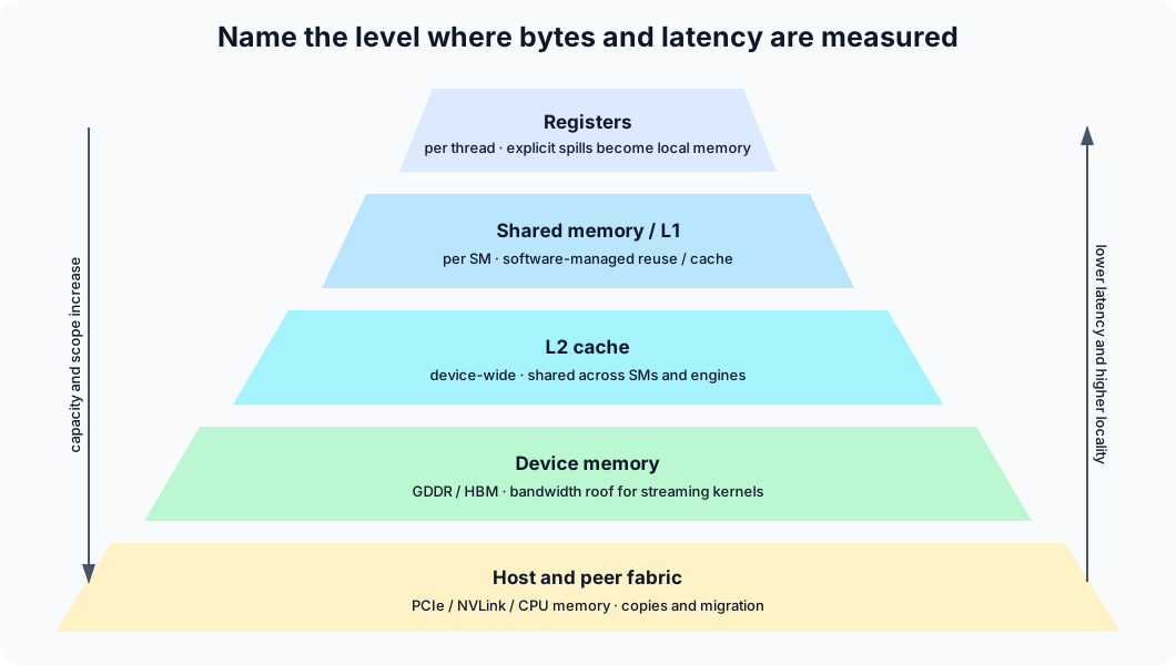
“Memory-bound” can describe bandwidth saturation, latency, poor transactions, cache thrashing, spills, or too little parallelism. These require different fixes.
Bandwidth and arithmetic intensity
Effective bandwidth is
Arithmetic intensity at a chosen hierarchy level is
The roofline bound is
Always name the byte level. DRAM arithmetic intensity and L1 arithmetic intensity are not interchangeable.
Explicit copies versus streaming kernels
“Memory-bound” also conflates explicit copies with traffic that kernel instructions generate on their own; separate the two before deciding what to optimize.
| Evidence | Meaning |
|---|---|
| red H2D/D2H/D2D activity in Systems | explicit CUDA memcpy or migration |
| high DRAM throughput inside a named kernel | load/store traffic generated by instructions |
| local-memory sectors in Compute | spills/stack traffic, not an API memcpy |
| quantize/cast/contiguous kernels | real kernels whose primary job is format/layout movement |
In a representative graph-replayed training trace, one input D2D copy per
microstep was negligible. The apparent “copy storm” was mostly quantization,
pointwise, and normalization kernels repeatedly streaming activation or weight
buffers. Optimizing cudaMemcpyAsync would not address that traffic.
Coalescing and sector utilization
On modern CUDA GPUs, warp requests are serviced in aligned sectors. Sectors exist because the memory controller and the cache hierarchy above it move data in fixed-size chunks regardless of how many bytes a thread actually asked for; there is no hardware path that fetches just the four bytes a thread wants. When a warp's 32 threads request small, scattered addresses, each request can still trigger a full-sector fetch, so the warp pays for many complete sectors while using only a handful of bytes from each — that is the physical reason low sector efficiency wastes bandwidth. Compare requested useful bytes with transferred sectors. If each local or global load uses only 1–4 bytes of a 32-byte sector, the cache and memory system moves much more data than the program consumes.
For useful bytes and transferred bytes ,
Low efficiency suggests changing lane-to-data mapping, vectorization, structure-of-arrays layout, or tail handling. High efficiency with saturated DRAM suggests reducing total bytes or fusing adjacent passes.
Vectorization deserves a concrete description rather than just a name in that
list. Vectorized memory access means loading or storing through a wider
type — float4, int4, or an equivalent 8- or 16-byte-wide access — so each
thread issues one instruction for one full, naturally aligned chunk instead
of two, four, or more instructions for scattered smaller pieces. This helps
in two distinct ways that are worth separating: it cuts the instruction count
feeding the LSU pipe, the same issue-pressure argument ch. 8 makes for
memory-bound stalls, and, when the underlying data layout is already
contiguous per thread, it directly raises by construction,
because a full-width aligned request is exactly what a sector fetch is built
to serve. Vectorization does not fix a fundamentally scattered or
misaligned access pattern — it makes an already-contiguous pattern cheaper to
issue, so confirm the layout supports it before reaching for wider loads as
the fix for a low sector-efficiency number.
Shared-memory bank conflicts
Sector efficiency governs global and local traffic; shared memory has an analogous, on-chip bottleneck. Shared memory is physically built from multiple independent banks precisely so that up to 32 simultaneous accesses — one per lane, one per bank — can be serviced together in a single cycle, rather than one address at a time. A bank conflict is what happens when two or more lanes in the same request address the same bank: the bank can only honor one of them per cycle, so the hardware serializes the colliding accesses into extra wavefronts instead of servicing the whole warp at once. Nsight Compute reports excessive wavefronts/conflicts for shared loads and stores.
The classic transpose fix pads a square shared tile:
__shared__ float tile[TILE][TILE + 1];
The extra column changes the bank mapping of column accesses. Verify rather than assuming: modern instructions, element widths, and architectures alter the exact pattern.
Padding is simple but wastes the padding bytes on every row and can waste more once tile widths grow or vector-width accesses are involved. High-performance library kernels more often reach for shared-memory swizzling: a permuted address mapping — an XOR or similar bit-manipulation of the address, chosen so that colliding indices are pushed to distinct banks — that avoids the same conflicts without giving up any shared-memory capacity to padding. The tradeoff is that a correct swizzle depends on the exact access pattern, element width, and tile shape, and hand-deriving one is easy to get subtly wrong in a way that only shows up as a wrong answer or a conflict that reappears under a different tile size. Rather than deriving swizzle arithmetic from scratch, verify a candidate swizzle against a known-good library implementation such as CUTLASS's shared-memory layouts, or use the library's layout directly.
A memory decision table
Combine bandwidth, cache, and stall evidence into one table before picking a fix:
| DRAM throughput | Cache hit | Long scoreboard | Likely next move |
|---|---|---|---|
| high | any | any | reduce bytes, fuse, compress, increase reuse |
| low | low | high | fix coalescing or increase memory-level parallelism |
| low | high | high | dependency chain or cache latency; add independent work |
| low | high | low | probably limited elsewhere; inspect compute/issue |
For a memory-bound activation kernel already sustaining roughly 89% of DRAM peak, micro-optimizing arithmetic has little ceiling. Fusion that avoids a read and write is the high-leverage experiment.
That "high DRAM throughput" row is also the signal that separates a kernel worth pipelining from one that is not. Once DRAM throughput confirms the kernel is actually bandwidth-bound rather than merely latency-stalled with bandwidth to spare, software pipelining — issuing the next tile's load before consuming the current tile's data, so load latency overlaps with compute on data already resident, as described in ch. 8's stall-to-fix section — is the technique that lets a kernel approach the DRAM ceiling instead of stalling between each tile's load and use. Pipelining does not reduce bytes moved, so it does not help the "reduce bytes, fuse, compress" row above; it helps a kernel spend the bytes it does move without adding idle cycles around each transfer.
10. Tensor Cores, shapes, and tile alignment
Tensor Core eligibility, Tensor-pipe saturation, and whole-device efficiency are separate questions.
Tensor Cores are specialized execution units on the SM, separate from the general CUDA cores that execute ordinary scalar and vector floating-point and integer instructions. They are built to perform small, fixed-shape matrix-multiply-accumulate operations directly in hardware, completing far more FLOPs per cycle than the same math expressed as ordinary instructions — but only for the specific data types, tile shapes, and memory layouts that a given MMA (matrix-multiply-accumulate) hardware instruction supports. This is why Tensor Core eligibility is a binary, all-or-nothing condition rather than a smooth efficiency curve: for a given operation, the compiler either emits a Tensor Core MMA instruction, or it falls back to ordinary scalar/SIMT instructions on the same data. There is no partial credit for an unsupported shape or dtype — the operation either fits the hardware instruction's fixed contract or it does not run on the Tensor pipe at all. That all-or-nothing behavior is why the rest of this chapter treats shape, alignment, and layout as correctness-for-performance questions rather than ordinary tuning knobs.
Shape the operation
For , useful work is
A tiled kernel launches approximately
CTAs. If is not a multiple of the number of simultaneously resident CTAs across the GPU, the last wave is partial.
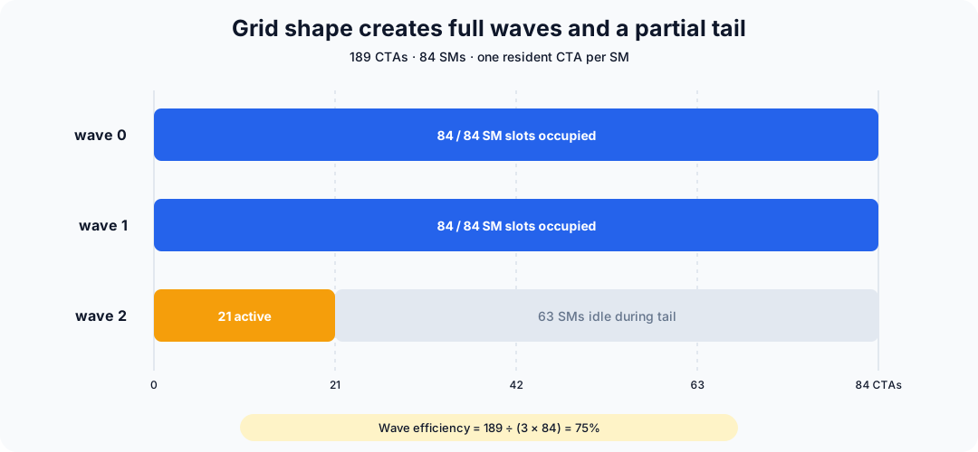
The approximate wave efficiency for SMs and CTAs/SM is
Padding efficiency
Wave efficiency is a device-level tail effect; padding efficiency is the per-tile analog inside each CTA. If a tile kernel computes padded dimensions , useful-work efficiency is
Alignment requirements depend on architecture, dtype, MMA instruction, and library. Record pointer alignment, leading dimensions, strides, and all three contraction dimensions; do not rely on a universal “multiple of 8” rule.
When shape alone can't fix wave efficiency
Wave efficiency and padding efficiency are both properties of the natural shape and the tile size chosen for it. Sometimes neither knob is enough: the shape itself does not produce enough CTAs to fill the device, no matter how the tile is chosen. Two named techniques exist for that case.
Split-K addresses a shape where and are small but is large — the grid formula from earlier in this chapter is computed from and alone, so a small-/large- problem can produce far fewer CTAs than the GPU can run concurrently, leaving most of the device idle regardless of tile shape. Split-K partitions the (reduction) dimension itself across additional CTAs, so each CTA computes a partial reduction over a slice of into a separate buffer, and a small combine/reduction pass afterward sums the partial results into the final output. This turns a grid that was too small to fill the device into one that is, at the cost of that extra combine step and the memory it touches — a cost worth measuring against the wave-efficiency loss it is meant to fix, not assumed to be free.
The persistent-kernel pattern — defined in ch. 8's stall-to-fix section as a grid sized to the device's resident-CTA capacity, with each CTA looping internally over the problem's tiles — is the other lever, and it addresses tail-wave loss directly rather than by reshaping the reduction. Because a persistent kernel's grid never depends on matching a multiple of , it has no partial last wave to lose efficiency to: the same resident CTAs simply keep pulling tiles until the problem is exhausted. This is the pattern behind most modern high-performance GEMM and attention kernels' near-full device utilization, and it composes with the warp-specialization and asynchronous-copy patterns described elsewhere in this chapter rather than replacing them.
Diagnose Tensor misalignment
Combine shape and padding effects with pipe utilization to tell a fed Tensor pipe from a starved one:
| Observation | Interpretation |
|---|---|
| no Tensor instructions; FP pipe busy | fallback path, unsupported dtype/layout/alignment |
| Tensor pipe high; runtime still poor | tile waves, epilogue, memory, or simply large work |
| Tensor and L2 both high | balanced kernel; probably not first optimization target |
| Tensor low; eligible warps high | instruction mix lacks enough MMA work |
| Tensor low; no eligible high | dependency/occupancy prevents feeding the pipe |
Check the exact selected library kernel and SASS instruction mix. For custom code, verify the compiler emitted the expected MMA family rather than scalar or SIMT fallback.
Warp specialization is not ordinary occupancy
Modern GEMMs often assign producer warps to asynchronous copies and consumer warps to MMA. Large register and shared-memory footprints enable deeper pipelines. Symptoms can include one CTA/SM, 17–25% achieved occupancy, sleeping producer warps, and yet 75–85% Tensor utilization.
Treating sleeping stalls or one-CTA residency as defects can dismantle the pipeline that makes the kernel fast. Compare alternative library tiles on the real shape instead.
Practical shape sweep
Once shape, padding, or specialization is suspect, measure rather than reason from formulas alone. Use a library profiler or microbenchmark to sweep neighboring dimensions and layouts:
cutlass_profiler --operation=Gemm \
  --m=4096 --n=4096 --k=4096 \
  --A=bf16:row --B=bf16:column --C=bf16 \
  --verification-enabled=true
Then test the selected implementation end-to-end. A standalone GEMM winner may lose after layout conversion or quantization overhead is included.
11. Source, PTX, and SASS correlation
Counters locate the limiting resource. Source and SASS identify the instruction responsible for it.
nvcc compiles CUDA C++ in stages rather than going straight to hardware
instructions. It first compiles to PTX, a portable virtual instruction set
that stays stable across GPU generations — conceptually similar to a portable
assembly language, but not the code the hardware directly executes. From
there, either at build time via ptxas or lazily at runtime by the CUDA
driver's own JIT compiler, PTX is lowered to SASS: the GPU's native,
architecture-specific machine instructions, the final compiled form actually
run by the hardware. Register allocation, instruction scheduling, and the
choice of which hardware instruction to emit — such as whether an MMA
instruction was actually generated for a given operation — are all decided
during this lowering step, not before it. PTX is one compilation stage
removed from what the hardware runs.
Build for correlation
For optimized profiling builds, prefer line information without full debug code generation:
nvcc -O3 -lineinfo -Xptxas=-v kernel.cu -o kernel
-G changes optimization and resource use substantially; reserve it for
correctness debugging. Keep generated cubins/cache files for JIT systems when
possible.
The lowering path
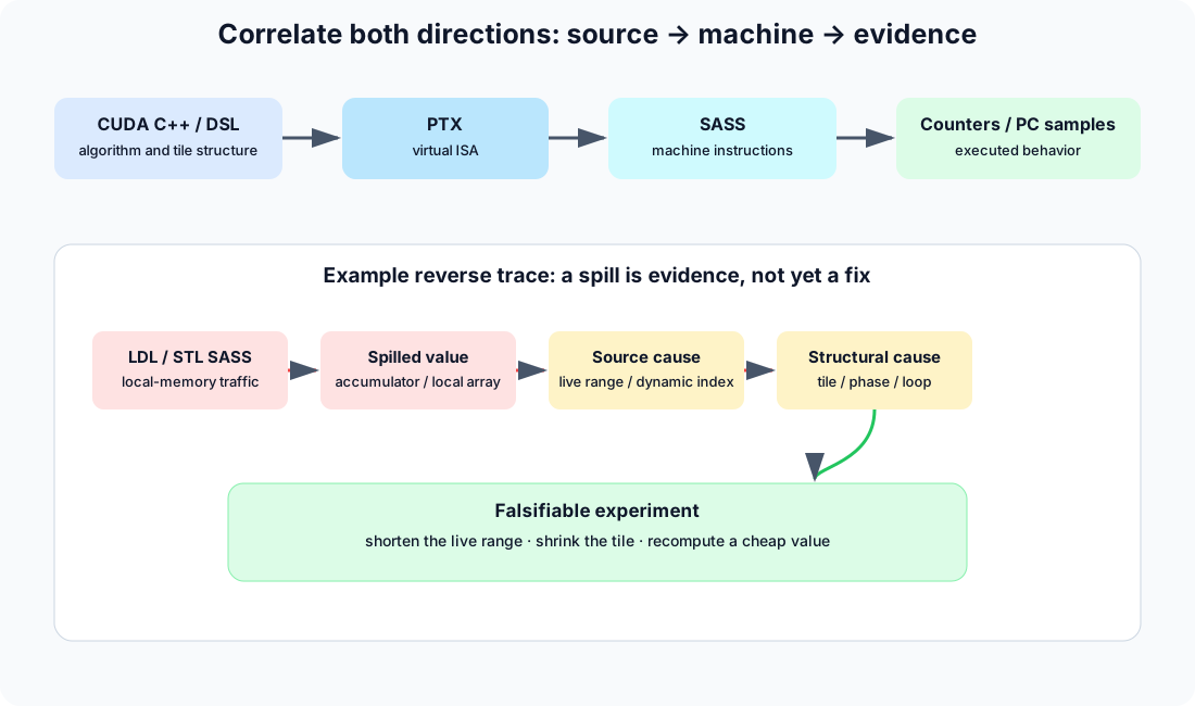
PTX is not the final instruction stream. Register allocation, instruction scheduling, memory operations, and Tensor instructions must be confirmed in SASS or Nsight Compute's Source page.
Command-line inspection
Confirm the lowering path directly, without the UI, when a quick check or a scripted comparison is enough:
cuobjdump --dump-resource-usage ./application
cuobjdump --dump-sass ./application
nvdisasm --print-line-info kernel.cubin
In Nsight Compute, correlate hot PCs and sampled stalls with both source and SASS. Look for:
- local loads/stores near long-scoreboard samples;
- repeated address arithmetic feeding LSU pressure;
- shared-memory operations with conflict wavefronts;
- missing or sparse MMA instructions;
- barriers and waits in a tight loop;
- type conversions or FP32 instructions in an intended low-precision path.
Source attribution can be incomplete
Header-only libraries, JIT kernels, stripped cubins, link-time code, and code generated without line info may show only SASS. The diagnosis is still possible: use instruction addresses, register dependency chains, opcode class, and memory spaces. Do not rebuild with radically different optimization flags and assume the new kernel represents production.
From sample to edit
Suppose long-scoreboard samples land on a local load. Trace backward:
- Locate the hot PC/source line on Nsight Compute's Source page.
- Confirm the instruction addresses local, not global, memory — check the memory space in the disassembly or the local-traffic counters, not just the opcode.
- Identify the register or variable whose live range or dynamic indexing forces the spill (see the register-spill diagnosis in ch. 7).
- Trace that variable to the source-level construct responsible: a large per-thread array, a live range spanning a loop, dynamic indexing into a local array, or excessive live temporaries.
- Form the one-variable experiment: change that single tile or live-range parameter and nothing else.
After editing, require the full chain to improve: fewer local sectors, more eligible warps or shorter dependency stalls, lower representative launch time, and lower end-to-end time.
12. Controlled performance experiments
A counter report should end in an experiment, not an adjective.
Write the hypothesis first
Use this form:
Because evidence, changing one mechanism should improve specific counters and reduce specific elapsed time, without changing correctness constraints.
Example:
Because a backward kernel is register-limited to eight active warps/SM and local-memory loads dominate its long-scoreboard samples, shortening the live range of the per-thread accumulator should reduce local sectors and no-eligible cycles, then reduce both kernel and iteration time.
Keep an experiment ledger
Turn each hypothesis into a row before running it, and keep every prior row instead of overwriting it — the ledger is what lets a later result be compared against the reasoning that motivated it:
| Revision | Workload | Change | Median | p20–p80 | Key counters | Correct? |
|---|---|---|---|---|---|---|
| baseline | M,N,K / batch,seq | none | … | … | … | yes |
| A | same | smaller tile | … | … | regs, spills, Tensor% | yes/no |
Do not combine tile size, precision, fusion, and launch geometry in one patch if you want to understand causality. Change several of them at once and a favorable result cannot be attributed to any one of them — an improvement without a known mechanism is a lucky patch, not the kind of causal, generalizable understanding of the kernel that lets you predict its behavior on the next shape or the next change.
A favorable median in the ledger is not yet a validated result — it still has to survive the same causal chain the hypothesis predicted, link by link.
Optimization proof chain
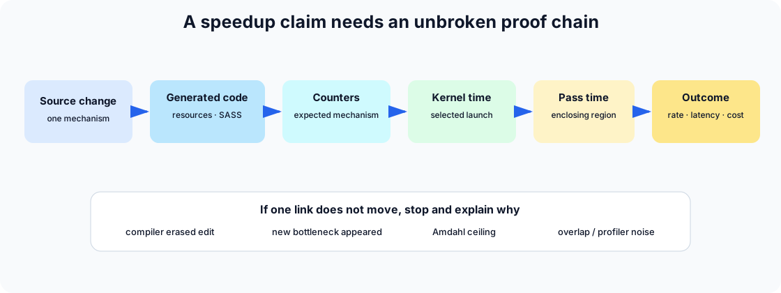
If the chain breaks:
- generated code unchanged: the compiler optimized away or restructured the edit;
- counters improve but kernel does not: another resource became limiting;
- kernel improves but pass does not: launch is too small or another shape dominates;
- pass improves but end-to-end does not: overlap or an outside bottleneck hides it;
- end-to-end improves only under profiler: measurement perturbation or noise.
A chain that holds end to end proves the change is fast. It says nothing about whether the change is still right, which is a separate and equally required check.
Correctness is multidimensional
For numerical kernels check representative distributions, edge shapes, non-contiguous layouts, tails, NaN/Inf behavior, deterministic requirements, and backward gradients where applicable. A faster reduced-precision path that changes convergence is an algorithm change, not a free kernel optimization.
Re-profile at the right level
A change that is fast and correct in isolation is still only a local win. After it lands, return to Nsight Systems. Removing one kernel can expose CPU gaps, shift library selection, change overlap, or make another family dominant. The profiling funnel is iterative.
13. Case studies
These case studies use a representative single-GPU, mixed-precision, approximately one-billion-parameter transformer training microstep. The batch contains 16 sequences of 1,024 predicted tokens. Activation checkpointing and CUDA Graph replay are enabled. The purpose is the diagnostic method; no knowledge of a particular model implementation is required.
Case A: thousands of launches, but not CPU-starved
A microstep launching several thousand kernels looks, on its face, like the textbook case for host-dispatch overhead — so that hypothesis is the one to rule in or out first, before trusting anything built on top of it. Ten graph replays contained 49,480 internal kernel nodes: 4,948 per microstep. The measured range was 12.810 s; the union was effectively serial and summed kernel time was 12.789 s. Device-idle time was therefore about 2.10 ms per microstep, or 0.164%.
| Observation | Superficial conclusion | Evidence-backed conclusion |
|---|---|---|
| 4,948 kernels/microstep | launch overhead must dominate | graph replay feeds them continuously |
long host cudaGraphLaunch calls | launch API is slow | calls block under queue backpressure while GPU runs |
| almost no device gap | — | CPU dispatch is not the current hot-path limit |
This does not prove the input pipeline will remain sufficient with real storage or distributed communication. It proves that kernel optimization, not further launch aggregation, controls this captured steady-state interval.
CUDA-event pass timing on the same shape makes the target more precise:
| Pass | Median stream time | Share | Median host enqueue time |
|---|---|---|---|
| backbone forward | 229.83 ms | 19.4% | 107.04 ms |
| fused vocabulary loss | 111.32 ms | 9.4% | 3.72 ms |
| backward + checkpoint recompute | 845.92 ms | 71.3% | 895.38 ms |
| total | 1,187.07 ms | 100% | — |
The host and stream columns are overlapping clocks, so they must not be added. Backward's long host enqueue interval says dispatch is close enough to monitor; the Systems trace's near-continuous GPU work says it is not presently opening meaningful device gaps. Backward and recompute own most of the optimization ceiling.
Whole-range GPU metric sampling supports the same conclusion:
| Sampled metric over three graph replays | Mean |
|---|---|
| graphics/compute engine active | 99.67% |
| at least one SM warp active | 93.29% |
| SM instruction issue | 19.02% |
| Tensor pipe active | 37.26% |
| compute warps in flight | 35.25% |
| DRAM read / write throughput | 33.89% / 21.84% |
| PCIe receive / transmit throughput | 0.22% / 1.01% |
The GPU is occupied, but the mixed workload does not continuously feed one execution pipe. Low PCIe activity also rules out host transfer bandwidth as the captured hot-path explanation. That low aggregate issue rate is a symptom, not a diagnosis — it describes no single kernel, and opening one of 4,948 launches at random would not explain it. It does not mean every kernel has 19% issue efficiency; it means the next step is to find where time actually concentrates before opening any one kernel.
Case B: identify the aggregate ceiling
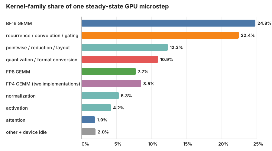
Attributing device time by kernel family, rather than by individual launch, answers that question directly: the workload is not dominated by one bad kernel. BF16 GEMMs are the largest family (24.8%), recurrent/convolution/gating kernels are close behind (22.4%), and format/layout work is distributed across pointwise and quantization families (23.2% combined).
Consequences from Amdahl's law:
- infinitely accelerating the recurrent family alone caps speedup at 1.289x;
- halving all quantization plus pointwise/layout work yields about 1.13x;
- reaching a 2.35x end-to-end target requires changing several large families or the hardware/parallelism, not polishing one kernel.
Format/layout and quantization work is one of those large families, and it is also the easiest to misjudge from a family label alone: on paper it looks like plain data movement, so the natural next question is whether it is actually copy traffic or compute wearing a copy's clothing.
Case C: “copy traffic” is mostly kernels
Quantization and pointwise/layout kernels made up nearly a quarter of the trace in Case B, so the question is what that share actually is. The trace showed only one small device copy per graph replay. By contrast, quantization kernels consumed 10.9%, and pointwise/reduction/layout kernels 12.3%. Two representative streaming kernels reached 88–89% DRAM throughput: a fused activation and a normalization kernel — each one is already efficient in isolation, so the excess time cannot be blamed on either kernel being slow.
The diagnosis is repeated read/transform/write passes, not a pathological
cudaMemcpyAsync. Useful experiments are fusion, reuse of quantized weights,
avoiding redundant layout materialization, or changing precision boundaries.
The activation arithmetic itself has little standalone ceiling when its kernel
already sits near the DRAM roof.
One FP4 packing kernel was different: 83% SM compute versus 35% DRAM, 100 registers/thread, and 33% theoretical occupancy. It is compute-heavy format conversion, so describing all quantization as “copying” would also be wrong.
That kernel's register count and occupancy are the first hint of a sharper, more specific problem than “too much traffic”: a kernel whose resource footprint limits how much work the SM can keep resident. The next case follows that thread to a single kernel where the full causal chain from registers to stalled scheduler cycles can be traced end to end.
Case D: maximum registers and spills are causal
A recurrent backward kernel represented 3.38% of the iteration by itself. It used 255 registers/thread with 128-thread blocks, achieved only eight warps/SM, generated 9.65 million local spill requests, and had no eligible warp on 91.6% of scheduler cycles. Long scoreboard accounted for 56% of its issue interval.
This is the clearest custom-kernel target because the causal chain is complete: register pressure reduces residency; spilling adds cache/memory dependencies; limited resident work cannot hide them; scheduler issue collapses. The first experiments should reduce live state or split a favorable phase—not impose a lower register cap.
A second backward kernel used 153 registers/thread, did not spill, achieved 25% occupancy, and reached 71% memory throughput. Its long-scoreboard latency is real, but it is a healthier, lower-priority memory-latency problem.
That contrast is worth generalizing before it is mistaken for a rule: low occupancy alone is not evidence of the first kernel's register/spill pathology. The next case checks that directly against two Tensor Core kernels that also run at moderate occupancy but are not register-limited at all.
Case E: low occupancy can be healthy
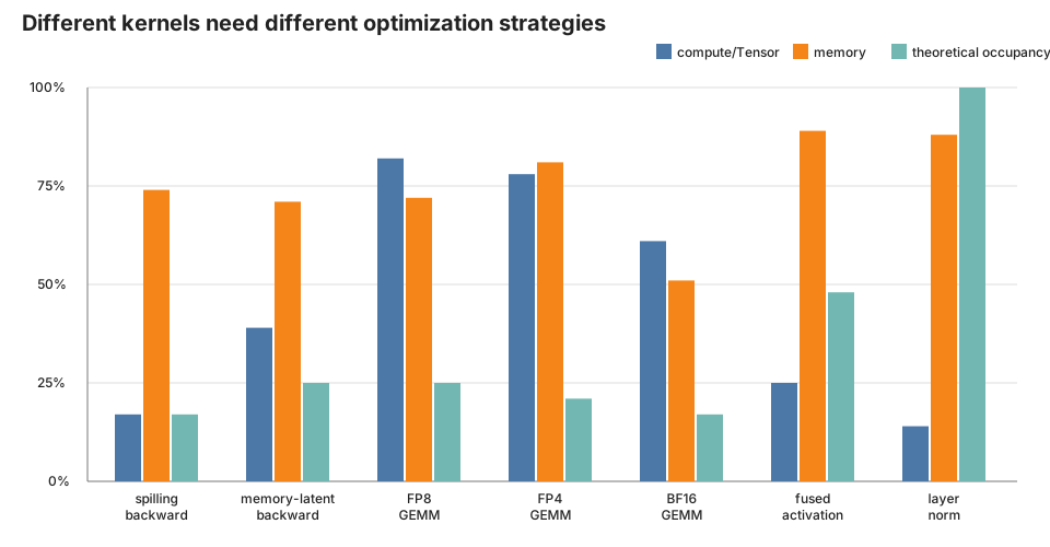
Neither depends on many resident warps to stay busy, so the question is whether their occupancy and stall numbers signal a problem to fix or a deliberate design already paying off. The FP8 GEMM reached about 82% Tensor-pipe utilization; the FP4 GEMM reached 78% Tensor and 81% memory/L2 throughput. Both deliberately ran one large, warp-specialized CTA per SM. Sleeping stalls represented producer/consumer waiting while the target pipelines remained busy.
The sampled grids also had efficient waves:
| Kernel | Grid CTAs | Assumed CTAs/SM | 84-SM wave efficiency |
|---|---|---|---|
| FP8 GEMM | 1,792 | 1 | 99.6% |
| FP4 GEMM | 4,736 | 1 | 98.9% |
| BF16 GEMM | 1,024 | 1 | 93.8% |
There is no evidence of a broad Tensor eligibility failure: the selected kernels execute Tensor instructions and saturate that pipe reasonably well. The BF16 sample is less efficient (61% Tensor, 51% DRAM, 16.7% occupancy) and shows math-pipe throttle without spills. Library tile selection and precision policy are more promising than rewriting the healthy FP8/FP4 kernels.
Cases A through E have now covered the aggregate picture and the specific kernel-level targets, both real (Case D) and illusory (Case E). One question remains that none of that kernel-level work answers: even capturing every identified gain, can this hardware reach the target at all?
Case F: feasibility before optimization
Answering that means comparing the measured rate against the actual target, not against intuition. The unprofiled steady-state baseline was approximately 14.08k tokens/s. A 20-tokens-per-parameter training budget for 1.0009B parameters is 20.018B tokens. Seven days therefore requires 33.10k tokens/s:
At the measured rate, the microstep-only lower bound is 16.45 days, before periodic optimizer, evaluation, checkpoint, or input costs. The gap is 2.35x. The profile shows no single-kernel route to that gain on this GPU. A realistic plan needs multiple GPUs or faster hardware, a smaller token/model budget, or a large algorithmic/precision redesign in addition to the identified kernel and fusion work.
None of that removes the value of the kernel and fusion targets identified in Cases B through E — it only bounds what they can accomplish alone. The final case runs those targets as an actual campaign and judges each one the way the rest of this book insists on: against whole-step time, not a counter in isolation.
Case G: a complete optimization campaign
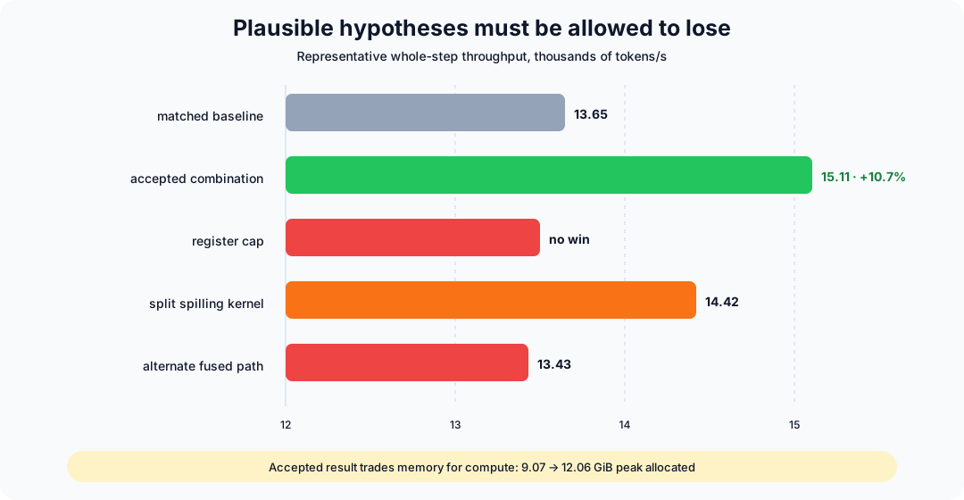
The same representative workload was used for a controlled campaign. The important result is not that every plausible counter-driven edit won. It is that every edit was allowed to lose, and only whole-step improvements survived.
| Hypothesis | Experiment | Result | Decision |
|---|---|---|---|
| eliminate one residual-sized memory pass | fuse residual addition with the following prenorm | about +3.2% in isolation | retain after numerical gradient comparison |
| duplicate quantization is avoidable | share a common activation quantization across two projections while preserving separate GEMMs | about +1.6% in an adjacent pair | retain; the twice-wide single GEMM selected a slower shape |
| spare memory can buy compute | retain four tail layers instead of recomputing them | largest local gain, about +9% in the sweep | retain; eight layers exceeded memory |
| some precision-tail work is unnecessary | reduce a four-layer high-precision tail to two | about +2.6% versus four in the sweep | retain; deleting the tail entirely regressed |
| occupancy is limited by 255 registers | cap registers at 128, 160, 192, and 224 | none beat uncapped | reject |
| spills justify splitting a backward kernel | materialize an intermediate between phases | numerically valid but slower | reject; added dot product and traffic outweighed spill savings |
The accepted changes interact, so their isolated percentages cannot be added. A matched 20-iteration comparison measured 13.65k versus 15.11k tokens/s:
Peak allocated memory rose from 9.07 to 12.06 GiB. That is not a regression in this experiment: memory below the device limit was intentionally exchanged for less recomputation. The decision would change if the production workload needed that headroom for optimizer state, communication buffers, or longer sequences.
The post-change graph made the traffic mechanism visible:
| Operation | Before / step | After / step | Change |
|---|---|---|---|
| common activation quantization | 120 | 84 | -30.0% |
| common transposed-activation quantization | 60 | 44 | -26.7% |
| all kernel nodes | 4,948 | 4,816 | -2.7% |
The small total launch-count change beside a large targeted count change is a useful reminder: the objective was not “fewer kernels.” It was fewer expensive full-tensor transformations while spending memory on avoided recomputation.
Finally, an instrumented post-change trace ran much slower than the unprofiled benchmark. Only bounded-range launch counts were compared across those reports; the end-to-end claim comes from matched unprofiled runs. This separation of evidence prevents profiler perturbation from becoming a false speedup or regression.
Read against the technique chapters, none of these six decisions is ad hoc.
Both accepted fusions — the residual/prenorm merge and the shared activation
quantization — are ch. 9's read-and-write elimination applied to concrete
GEMM neighbors once DRAM throughput was already high. The accepted
precision-tail reduction is ch. 8's Math Pipe Throttle lever of routing more
work onto a cheaper Tensor Core precision, bounded by ch. 10's dtype-eligibility
contract for whichever MMA path is actually available. Both rejections fail
for reasons the earlier chapters already flag: capping registers is the blind
-maxrregcount move ch. 7 warns against, and materializing an intermediate
between phases is exactly the kernel-split experiment ch. 7's spill diagnosis
suggests trying — it loses here because the added dot-product and traffic cost
is the accounting ch. 9 asks for before trusting a spill fix. The
warp-specialized FP8/FP4 GEMMs from Case E are what ch. 8's persistent-kernel
pattern and ch. 10's warp specialization look like once they are already
paying off, which is why this campaign's remaining slack was memory and
precision policy around them, not occupancy.
14. External practice exercises
Use these small workloads to learn one phenomenon at a time before profiling a large application.
1. Vector addition: bandwidth and launch overhead
Vector addition is close to the simplest kernel that can exist: one load, one add, one store, no data reuse, no branching. That is precisely why it is the right starting point — any launch-overhead or bandwidth-roof effect seen here cannot be blamed on algorithmic complexity, so it isolates the profiling phenomenon itself rather than an artifact of the workload.
Profile C[i] = A[i] + B[i] across sizes from 1 KiB to 1 GiB.
Predict and then verify:
- small sizes are launch/latency dominated;
- large sizes approach a DRAM bandwidth roof;
- effective bytes are two reads plus one write;
- occupancy beyond what hides memory latency does not raise the roof.
Start from the official CUDA Samples repository's introductory vector example or write a one-dimensional grid-stride loop.
2. Matrix transpose: coalescing and bank conflicts
Vector addition isolated a single memory pass in one dimension. Transpose adds a second dimension and a shared-memory path, which is what makes it possible to tell coalescing and bank-conflict effects apart.
Implement three versions:
- direct transpose with strided stores;
- shared-memory tiled transpose;
- tiled transpose with a padded shared leading dimension.
Use Systems to confirm equal launch structure, then Compute to compare global sector efficiency, shared conflict wavefronts, and effective bandwidth. This is the cleanest exercise for separating DRAM transactions from shared-memory bank mapping.
3. Reduction: synchronization and tail behavior
Transpose kept every thread's work independent until the final store. Reduction removes that independence: threads must combine results, so synchronization and tail behavior become the new variable to isolate.
Sweep power-of-two and awkward sizes. Compare a block reduction with a warp-shuffle version. Inspect barrier stalls, branch efficiency, waves, and the cost of a second reduction launch. Then test whether fusion into the consumer beats a locally faster standalone reduction.
4. GEMM: Tensor eligibility and waves
The first three exercises are memory-bound by construction. GEMM moves the ceiling to the Tensor pipe, where eligibility and wave efficiency replace DRAM throughput as the limiting question.
Use the CUTLASS Profiler or cuBLAS benchmark to sweep neighboring values, dtypes, and layouts. Record selected kernel, Tensor-pipe utilization, tile count, wave efficiency, and padding efficiency. Include small skinny matrices; square peak-TFLOP charts do not represent every application.
5. Fused softmax or layer normalization: the fusion roof
GEMM isolated one large compute-bound kernel. Fusion goes the other way, asking how many of the smaller memory-bound passes from exercises 1 and 3 can be collapsed into one kernel instead.
Compare a framework composition with the official Triton fused-softmax or layer-normalization tutorial. Count launches and bytes avoided. A successful fusion should show both a simpler Systems timeline and less memory traffic, not merely fewer source lines.
6. Attention: resource trade-offs
Attention is where the earlier lessons compound: Tensor Core eligibility (exercise 4) and kernel fusion (exercise 5) now share one kernel with the register and occupancy limits from the transpose and reduction exercises.
Use the Triton fused-attention tutorial across head dimensions and sequence lengths. Track register count, shared memory, occupancy, Tensor utilization, and numerical correctness. Observe how the best tile changes with shape and how an occupancy decrease can accompany a speedup.
Each exercise should produce a one-page ledger: baseline, hypothesis, one change, relevant counters, selected-kernel timing, and end-to-end timing. This is the same ledger discipline from chapter 12, applied to workloads small enough to iterate on in minutes rather than hours.
15. Command and metric reference
Commands are templates. Check --help because Nsight options and report names
evolve.
Baseline inventory
Record the hardware and tool versions before any profiling run:
nvidia-smi -L
nvidia-smi --query-gpu=name,driver_version,pstate,clocks.sm,clocks.mem,\
temperature.gpu,power.draw,memory.total --format=csv
nsys --version
ncu --version
Nsight Systems
Capture a bounded CUDA/NVTX timeline:
nsys profile --trace=cuda,nvtx,osrt \
  --sample=process-tree --cpuctxsw=process-tree \
  --output=timeline ./application
Expose nodes inside CUDA Graphs when necessary:
nsys profile --trace=cuda,nvtx \
  --cuda-graph-trace=node --output=graph_nodes ./application
Sample GPU metrics on supported systems:
nsys profile --trace=cuda,nvtx \
  --gpu-metrics-device=all \
  --gpu-metrics-frequency=10000 \
  --output=gpu_metrics ./application
Generate summaries:
nsys stats --report cuda_gpu_kern_sum,cuda_gpu_mem_time_sum timeline.nsys-rep
nsys stats --report cuda_api_sum,nvtx_sum timeline.nsys-rep
nsys stats --report cuda_gpu_trace:base timeline.nsys-rep
Nsight Compute
List sets and sections:
ncu --list-sets
ncu --list-sections
ncu --query-metrics-mode suffix --metrics sm__throughput
Profile exactly one matching launch (replay makes each additional launch costly, and a later launch may not represent the shape or state you actually want to characterize):
ncu --set detailed \
  --kernel-name-base function \
  --kernel-name 'regex:kernel_name' \
  --launch-count 1 \
  --output=kernel_report \
  ./application
Reach the sixth matching launch:
ncu --set full --kernel-name 'regex:kernel_name' \
  --launch-skip 5 --launch-count 1 -o kernel_sixth ./application
Collect selected sections:
ncu --section SpeedOfLight \
  --section LaunchStats \
  --section Occupancy \
  --section SchedulerStats \
  --section WarpStateStats \
  --section MemoryWorkloadAnalysis \
  --section ComputeWorkloadAnalysis \
  --section SourceCounters \
  -k 'regex:kernel_name' -c 1 -o focused ./application
Export details:
ncu --import focused.ncu-rep --page details --csv
Compilation and disassembly
Build with line info, not full debug info (-G disables optimizations and
changes the generated code), and inspect the generated code directly:
nvcc -O3 -lineinfo -Xptxas=-v kernel.cu -o kernel
cuobjdump --dump-resource-usage ./kernel
cuobjdump --dump-sass ./kernel
nvdisasm --print-line-info kernel.cubin
Metric map
Use section labels in the UI before relying on raw metric names. Raw names are architecture-specific, but their prefixes are useful:
| Prefix | Unit or concept |
|---|---|
sm__ / smsp__ | SM / SM subpartition, schedulers and instruction issue |
dram__ | device-memory traffic/throughput |
lts__ | L2 cache slices |
l1tex__ | L1/TEX/shared-memory path |
sass__ | executed SASS instruction/source metrics |
launch__ | static/dynamic launch attributes |
Minimal interpretation worksheet
Fill this in, in order, for any kernel under investigation:
Workload and shape:
End-to-end metric and distribution:
Pass / family share:
Selected launch (grid, block, regs, smem):
Compute vs memory throughput:
Theoretical / achieved occupancy:
Active / eligible / issued warps:
Dominant stalls (only if issue-starved):
Bytes, hit rates, sectors, local traffic, conflicts:
Dominant execution pipe and expected instructions:
Source/SASS location:
Amdahl ceiling:
Next one-variable experiment:
16. Troubleshooting and counter access
ERR_NVGPUCTRPERM or no permission for counters
Recent NVIDIA drivers restrict access to GPU performance counters by default. On a workstation, enable access through the NVIDIA settings UI:
- NVIDIA App: System → Advanced → Developer → Manage GPU Performance Counters, then allow access for all users.
- Legacy NVIDIA Control Panel, run as administrator: enable Developer Settings, open Developer → Manage GPU Performance Counters, and allow access.
On Linux, an administrator can instead grant only the profiling process the required capability or configure the driver's counter-access policy. Follow NVIDIA's current platform-specific instructions rather than copying an old module option blindly. Containers must pass through the profiling capability as well as the GPU.
Verify with a one-launch basic capture:
ncu --set basic --kernel-name 'regex:known_kernel' \
  --launch-count 1 ./application
On WSL, restart the WSL VM after changing Windows driver settings if access does not update immediately:
wsl --shutdown
Nsight Compute cannot connect to the CUDA driver
Check that the process sees the real driver library rather than the CUDA stub:
nvidia-smi
ldconfig -p | grep libcuda
Containers need GPU device access and profiling permissions. A sandbox may intentionally block the driver even when ordinary shell CUDA programs work.
System-wide CPU sampling fails
Linux perf_event_paranoid, container capabilities, or WSL support can block
system-wide samples. Prefer process-tree sampling when it answers the question:
nsys profile --sample=process-tree --cpuctxsw=process-tree ./application
Lowering a system security control is an administrative decision, not a routine profiling step.
Reports disagree on duration
Expected causes include warm-up, clock variation, ncu multi-pass replay,
memory backup/restore, cache-state changes, graph tracing mode, and profiler
overhead. Use:
- unprofiled wall time for final performance;
- Systems for pass/family contribution and gaps;
- Compute for per-kernel character;
- a microbenchmark with stable clocks for precise kernel comparisons.
Achieved occupancy looks impossible
Very short kernels, periodic sampling, new architectures, or tool/driver version mismatches can produce counter anomalies such as achieved occupancy slightly above the nominal maximum. Cross-check static theoretical occupancy, active-warps counters, duration, and release notes. Do not anchor a rewrite on one implausible sampled value.
Source correlation is missing
Rebuild the production-equivalent optimized binary with -lineinfo, retain JIT
artifacts, and ensure Nsight Compute can locate source paths. Avoid -G for
performance characterization. If only SASS is available, profile by PC and
opcode class.
Profiling takes forever
Full-application replay-based profiling scales with what the kernel touches, not just how long it runs. Narrow the scope before accepting a long capture:
- filter one exact kernel occurrence;
- begin with
basicor selected sections; - shorten the workload after warm-up;
- use NVTX/start-stop ranges;
- consider application/range replay for large touched memory or stateful code;
- disable source/PC sampling sections until needed.
The GUI cannot open a remote report
Capture with CLI on the target, copy the .nsys-rep or .ncu-rep, and open it
with a compatible or newer desktop UI. Preserve reports alongside version and
command metadata.
Further reading
NVIDIA profiling tools
- Nsight Systems User Guide — capture modes, CUDA/NVTX tracing, CPU sampling, GPU metrics, and CLI options.
- Nsight Systems post-collection analysis — reports, recipes, and trace export.
- Nsight Compute documentation — UI, CLI, profiling guide, and developer interfaces.
- Nsight Compute Profiling Guide — replay, metric semantics, scheduler states, occupancy, rooflines, and stall reasons.
- Nsight Compute CLI Guide — filtering, sections, NVTX, multi-process profiling, and report import.
- NVIDIA performance-counter permissions — current Windows, Linux, container, and platform instructions.
CUDA architecture and optimization
- CUDA C++ Programming Guide — execution model, memory hierarchy, synchronization, and architecture features.
- CUDA C++ Best Practices Guide — coalescing, bandwidth, occupancy, register pressure, NUMA, and optimization process.
- CUDA Binary Utilities —
cuobjdump,nvdisasm, instruction-set reference, and resource usage. - NVTX documentation and source — application semantic ranges and domains.
- CUDA Samples — bandwidth, matrix, graph, and performance examples.
Kernel libraries and DSLs
- CUTLASS Profiler — enumerate and benchmark GEMM/convolution implementations and shapes.
- CUTLASS quickstart — architecture-specific build and profiler configuration.
- Triton tutorials — vector add, fused softmax, GEMM, normalization, attention, and block-scaled matmul.
- Triton matrix multiplication — tiling, grouped program ordering, L2 reuse, and autotuning.
- PyTorch profiler and autograd NVTX annotations — framework-level attribution before kernel analysis.
Kernel engineering technique guides
- How to Optimize a CUDA Matmul Kernel for cuBLAS-like Performance — a worklog that pairs each optimization step (coalescing, shared-memory tiling, vectorization, warp tiling) with its measured throughput against cuBLAS; a model for the diagnosis-technique-measurement loop this book itself follows.
- FlashAttention: Fast and Memory-Efficient Exact Attention with IO-Awareness — Dao et al.'s IO-aware attention algorithm; a well-known worked example of spending memory and recomputation to avoid a bandwidth-bound pass, the same trade-off ch. 13's Case G makes on this book's own representative workload.
- Programming Massively Parallel Processors: A Hands-on Approach (Hwu, Kirk, and El Hajj) — the standard foundational textbook for CUDA kernel-writing technique, from the memory model through tiling and tensor cores.
- Efficient GEMM in CUDA — CUTLASS's own account of hierarchical tiling, double buffering, and split-K/sliced-K reduction; the design rationale behind the library the Profiler doc above only benchmarks.
Suggested reading order
This list retraces the book's own funnel through the primary documentation: system-level tracing first, then one kernel, then the memory/occupancy and SASS layers underneath it.
- Nsight Systems CUDA trace and NVTX chapters — the system-level view Part I builds on.
- Nsight Compute sections, scheduler states, and replay — the per-kernel toolkit from Part II.
- CUDA Best Practices memory/coalescing and occupancy chapters — the mechanisms behind those Part II counters.
- A transpose exercise, then a GEMM shape sweep — the same coarse-to-fine method applied by hand.
- Source/SASS correlation on one custom kernel — the finest grain the funnel reaches.
- Simon Boehm's CUDA matmul worklog — once a target kernel is identified, a full worked sequence of implementing and measuring the fix, not just diagnosing it.
Documentation moves with toolkit releases. Prefer the version matching the installed tools when metric names or CLI syntax differ.